Grounded World Models: Efficient and Verifiable Structural Causal Prediction
Rafael Kaufmann, Harald Strömfelt, Thomas Minter, Sandeep Ramesh
Abstract
Investment decisions require predictive forecasts under hypothetical interventions which are coherently justified by the sum of available evidence. We argue this problem class selects a model class: the grounded world model (GWM), a verified, composable causal model whose every prediction is a Bayesian posterior under an explicit mechanism. We formalize GWMs and compare them theoretically and empirically with the default alternative: directly prompting a large language model (LLM) for predictions. Theoretically, we establish dominance results along both the efficiency and quality axes, which compound. Empirically, we benchmark Primordia’s investment GWM against a SOTA LLM (Claude Opus 4.8) on a standard investment analysis task. We show that GWMs’ explicit mechanistic, theory-aligned structure allows for \sim\!10^{5}\times parsimony compared to general-purpose LLMs, enabling incremental prediction at \sim\!36{,}000\times lower cost and \sim\!350\times lower latency, while achieving \sim\!2.4\times greater quality. Further, we show that any LLM predictor’s quality stays below the GWM’s at any finite cost, with cost per prediction diverging as that shared ceiling is approached. We propose a hybrid neurosymbolic structure—GWM as predictor, LLM as natural-language interface and query orchestrator—as the theoretically and empirically superior architecture for investment and other high-stakes real-world decision domains.
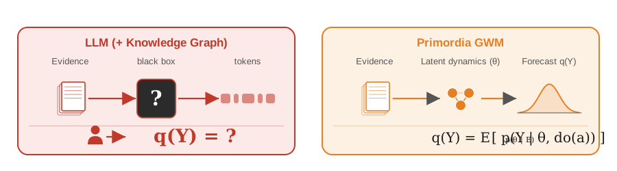
Figure 1: From narration to a grounded posterior. An LLM (even with a knowledge graph) answers a query with a prediction q(Y) that is not constrained to be any posterior—ungrounded and not auditable. A GWM casts a prediction as a proper Bayesian posterior under a causal generative model—grounded, source-traceable, and cheap.
1 Introduction
What does real-world, high-stakes decision-making require? The question is increasingly urgent, as we are rapidly offloading consequential decisions to “agentic” AI systems engineered around large language models (LLMs). The quality of those decisions is bounded by the capabilities of the systems sitting underneath them, and their cost is set by how those capabilities are achieved. Today the dominant answer is scale: more powerful models, longer reasoning traces, larger contexts, more agents reviewing other agents. The result is a cost/capability tradeoff that defines the practical application frontier of general-purpose LLMs. One might accept this tradeoff as the natural price of good decisions, but the history of prediction-intensive practices suggests an alternative path forward.
Consider how the practice of building a physical structure has matured. Building has one fundamental requirement, simply stated: the structure must stand. Whether a builder will succeed at this task depends in a highly specific way on their skill at predicting what will happen to the structure, during the building process and thereafter during its lifetime, under a wide variety of conditions and variations—a vast, implicit chain of “what-ifs”, many of which cannot be resolved definitively in advance, resulting in an extraordinarily peaked loss function. A child devises experiments using folk physics and builds by trial and error—enough for a tower of blocks, hopeless for anything long-standing. A medieval master builder drew on generations of accumulated heuristics: this affords far more complexity, but little adaptivity once circumstances depart from precedent. A structural engineer in the pre-computer era solved the governing equations by hand—genuinely predictive, but only as far as one expert can hold the procedural knowledge in their head: which equations to solve, which parameters matter, how to estimate them. And today, a builder who declines to use a CAD system—pre-loaded with scientifically validated models and parameters for every context, able to simulate a design in instants—is committing malpractice. And a “vibe-building” LLM-based system that purported to help with construction by retrieving heuristics and “reasoning through” the problem with mental math, however fast, would be considered an impressive demo of LLM capabilities, but for real work, such a system would necessarily have to offload the critical physical computations to a CAD engine.
The application of AI is quickly moving from simple, point-in-time decisions under extensive human supervision to autonomous, temporally-extended professional decisions, many of which interact with and impact partially-observable real-world systems, with running costs and serious risks. Yet in many such domains—investing, policy, operations—the state of the art still consists of accumulated heuristics and hand-solved models, held in expert heads. So long as humans hold responsibility and accountability for those decisions, they buffer against error with padding and oversight; but as their judgment is automated away by LLM-powered workflows in the name of efficiency, those buffers go with it. Delivering on the efficiency promise then requires a quality bar high enough to prevent catastrophic failures, at an operating cost low enough to justify the ROI.
Indeed, quality shortfalls are the largest driver of cost: an ungrounded prediction that is wrong—or merely unauditable—triggers verification and rework that compound downstream, so the true cost of a cheap answer is dominated by what happens after it is emitted. Conversely, the prevailing remedy for quality is to spend more inference, driving cost per decision up the frontier. For a one-off, low-stakes question, this bargain may be acceptable; but professional decision-making consists of repeated, high-stakes, evidence-coupled predictions, and there the tradeoff bites hardest exactly where it can least be afforded. This raises the question of whether the tradeoff is fundamental, or an artifact of the model class being asked to do the predicting.
We propose that the key capability required in these settings is structural causal prediction: (i) simulating the system forward under assumptions or hypothetical interventions (“what happens to this company’s free cash flow if the data-center build-out slows?”) and (ii) revising those forward simulations coherently as evidence arrives (“a supplier just guided down; update everything downstream”). Simulate-forward and condition-on-evidence are the defining operations of a causal generative model— what the CAD system does for the builder and the engineer-by-hand could only approximate.
We note that this capability is quite distinct from fluency, coherent-sounding reasoning, long-running memory, theoretical knowledge, mathematical problem-solving prowess, or any of the other capabilities identified heretofore in LLMs. An LLM can describe such a model in prose, and with a coding tool or spreadsheet it can even assemble and run an ad hoc one; what it cannot do is be one, because its outputs are not constrained to be the posterior of any explicit mechanism.[3]
Motivated by the above, we define a grounded world model (GWM) as a causal generative model of a domain whose structure mirrors the domain’s actual entities and mechanisms, whose parameters are grounded—tied to evidence by explicit, auditable inference—and which supports the two operations above natively: it can be intervened upon (simulate-forward) and conditioned on incoming evidence (condition-on-evidence) to return a calibrated posterior. What makes a model a GWM is this functional contract, not any particular implementation. A probabilistic program is one natural realization, and the one we use; but a GWM may equally be expressed as a structural causal model, a system of dynamical equations, or a simulator equipped with a likelihood—any representation that supports verified intervention and conditioning qualifies.
Fully-fledged GWMs already exist. Numerical weather prediction replaced expert pattern-matching with forward simulation of a grounded physical model, continuously corrected by assimilating observations—the “quiet revolution” (Bauer et al., 2015) that has gained roughly a day of forecast lead time per decade. We believe the same move can be brought to other domains, particularly business and finance; this belief motivated Primordia’s GWM for equity investing.
The difference in aims between GWMs and LLMs—GWMs directly predict real-world observables; LLMs predict token sequences in response to a decision-maker’s prompts, which can then be interpreted by her as predictions of the world—is reflected in architectural and engineering differences. Most strikingly, LLMs are generically underdetermined (hence the “L”), monolithic, dense, static, and stateless, while GWMs are parsimonious, modular, sparse, dynamic, and stateful (they update as the world changes). A GWM’s development and maintenance process is therefore rather different than an LLM’s, especially when (as in our case) complete mechanistic explainability is required. Primordia’s approach is based on a combination of continual, automated program synthesis, continual validation of predictions against outcomes, and expert-informed structural priors.[2000]
This paper aims to formalize the category of GWMs, to demonstrate that they dominate “LLMs-as-predictors” jointly on cost and quality—escaping, rather than optimizing along, the LLM cost/capability tradeoff—and to benchmark Primordia’s GWM implementation against a typical “LLM-as-predictor” workflow that a principal would otherwise deploy. We draw the running example from investment analysis, where Primordia offers a GWM-based platform since December 2025; but the argument is about the model class, and we flag its domain-independence throughout.
1.1 The thesis
1. Structural causal prediction requires a GWM. We define the task category and show that it requires a GWM (Section 2). LLMs and knowledge graphs fail to meet the requirements for structural reasons, not for want of scale—indeed, the prior probability that a language model’s circuit happens to implement exact conditioning decreases with parameter count (Proposition 3, Corollary 2).
2. LLM predictors’ explanation quality has a structural ceiling. A prediction is only as useful as the explanation behind it. We operationalize explanation quality (XQ) from observable, mechanism-checkable properties and prove it lower-bounds prediction quality (closeness to the ideal predictor), so a rational agent trusts a prediction in proportion to its XQ (Section 2.7, Proposition 1). An LLM predictor’s XQ has a ceiling strictly below the GWM’s, and no added inference budget can clear it, whereas the GWM sits at its conditioning-limited ceiling at flat cost in the quality target (Section 3).
3. GWM prediction is cheap, quickly amortizing build costs. Because a GWM answers each query by inference on a structure-aligned model rather than by a fresh narration, it is both far smaller and far cheaper per prediction than an LLM, and its one-time build cost is recovered within a handful of predictive distributions (Section 3).
1.2 Related work
World models.
LeCun (2022) argues that autonomous intelligence requires a learned world model supporting prediction and planning. We sharpen “world model” to the verified, parametric, causally-transparent causal model required by structural causal prediction, and contrast it with the implicit, unverified world model latent in an LLM. The GWM is the “symbolic” half of the neurosymbolic architecture in Garcez and Lamb (2023); Garcez (2025), with the LLM as the “neural” half; more broadly, Chiatti et al. (2026) argue that systematic neural/symbolic integration, not scale alone, is the route to reliable AI in critical domains, and the GWM is one concrete, deployed instance. Closest in spirit is Wong et al. (2023), who translate natural language into probabilistic programs (a “probabilistic language of thought”); we take the further step of grounding, verifying, and composing such programs into reusable foundation-model capital. This paper builds directly on our own prior work, Kaufmann et al. (2025), which introduced the pre-synthesized grounded world model—a synthesized, continually-refined probabilistic program supporting full Bayesian inference—and showed it reaching Bayes-optimal accuracy on a synthetic-equities benchmark where SOTA LLMs plateau near 40%; here we formalize the GWM as a model class and benchmark its cost and quality against narrative-world-model baselines. The GAIA tech tree (Walters et al., 2025b) instantiates the same neural/symbolic split—the LLM exploring, the verified model library serving as the symbolic half it retrieves from—for the domain of technology planning. Closely related in stance is the Scientist AI program of Bengio et al. (2025a): a non-agentic world model that generates theories to explain data, paired with an inference machine carrying explicit uncertainty, proposed as a run-time safety guardrail whose Bayesian risk bounds can reject dangerous actions (Bengio et al., 2025b). A GWM is a domain-specific, verified realization of exactly this “model that explains rather than acts” posture. Finally, using a GWM for control (Section 4.1) is active inference (Friston et al., 2017): acting to minimize expected free energy under a generative model.
Causality and probabilistic graphical models.
The GWM can be seen as a structural causal model (Pearl, 2009), which we represent as a probabilistic program (Koller and Friedman, 2009). That a causal model is necessary, not merely convenient, is established by Richens and Everitt (2024): any agent satisfying a regret bound under a large set of distributional shifts must have learned an approximate causal model, converging to the true model for optimal agents. We take this as the formal warrant for selecting the GWM by requirements.
Retrieval-, tool-, graph-, and memory-augmented LLMs.
A rapidly expanding family of systems equips an LLM with external structured knowledge or capabilities: knowledge-graph question answering (Baek et al., 2023; Edge et al., 2024); long-context retrieval (Lewis et al., 2020); “agentic memory” stores that accumulate and re-read facts across calls (Packer et al., 2023); and tool-augmented agents that call a calculator, spreadsheet, or code interpreter to compute rather than merely retrieve (Schick et al., 2023; Yao et al., 2022; Gao et al., 2023). The retrieval and memory members of this family share a ceiling regardless of sophistication: absent an explicit mechanism, they improve only the evidence an LLM can cite, so the model still narrates a forecast rather than computing one, gaining neither the grounding and auditability of a GWM nor proper Bayesian updating as evidence arrives. Consistent with this, Vals AI (2026) benchmarks tool-augmented SOTA LLMs on analyst-grade financial research and finds they plateau well short of reliability, even given unlimited test-time budgets.[3]
Computation-augmented LLMs.
A computation tool (i.e., code execution) is different in kind. Raising explanation quality with such a tool means using it to construct, on the fly, the very object we formalize: an explicit mechanism the LLM can condition on and re-query, i.e. an ad hoc GWM assembled at inference time. This is not a counterexample to our thesis but an instance of it: the rational endpoint of tool-augmentation, pushed far enough, is exactly the Mode-2/Mode-3 coupling of Section 4.1, where the LLM frames and explains while a verified model computes the posterior—a per-query, un-amortized version of the architecture we propose building once and reusing. Tellingly, the harness in (Vals AI, 2026) does not supply code-execution tools, foreclosing that path by construction.
Mechanism-embedding and explanation-extraction alternatives.
Two neural-side programs each share one property of a GWM while lacking the others. Physics-informed machine learning (Karniadakis et al., 2021) shares the commitment to mechanism, regularizing a network with known governing equations; but the result is a neural surrogate whose outputs remain unverified and whose evidence-absorption is not Bayesian conditioning, whereas a GWM keeps the mechanism an explicit program and its updates exact. Post-hoc explainability instead shares the aim of explanation: a large literature extracts accounts from a trained black box, ranging from local attribution (Ribeiro et al., 2016; Lundberg and Lee, 2017) to global, model-level counterfactuals (Sobieski and Biecek, 2024); a GWM inverts this, since its explanation is the mechanism and requires no extraction (Section 2.7).
Complexity economics.
Farmer (2024) argues that economics should make the move meteorology made—from equilibrium and reduced-form statistics to mechanistic, agent-level simulation—and conjectures that economic systems may be more tractable than the weather. We operationalize that program for structural causal prediction and take up the tractability conjecture in Section 4.
1.3 Roadmap
Section 2 builds a taxonomy of world models, defines the GWM and its grounding map, fixes its defining properties, positions it against alternatives, and formalizes prediction and explanation quality (proofs in Appendix G). Section 3 presents benchmark results, pricing the cost of a single grounded prediction, the cost to reach a target explanation quality, and the volume-and-lifetime costs. Section 4 consolidates the foundation-model, leverage, parsimony, and usage-mode discussion together with the groundedness ladder, generalization and the tractability hypothesis, and limitations; Section 5 concludes. Appendices define the explanation-quality components (Appendix C), work a single case end to end (Appendix E), collect the cost-model details (Appendix F) and the proofs including the XQ class ceilings and GWM dominance (Appendix G), and tabulate the symbol, value, and provenance of every numeric input (Appendix I).
2 The Grounded World Model, Formally
2.1 A taxonomy of world models
Fix a single observable system and an agent that must predict it. The weakest useful object is a machine that emits predictions; we sharpen “machine” in four steps, each adding a property that a later benchmark will price.
Definition 1 (World model).
A world model (WM) is any machine \mathcal{W} that, in a given internal state, samples point predictions \hat{y}\sim\mathcal{W} of an observable Y.
Definition 2 (Proper world model).
A WM is proper if in every internal state its samples are draws from a single coherent predictive distribution (PD): there is a probability measure q(Y) such that the queried samples are exchangeable with empirical law converging to q, and q obeys the probability axioms.
A WM that is not proper has no well-defined q: repeated queries need not be mutually consistent, and there is no object on which to compute calibration or divergence.
Definition 3 (Grounded world model).
A proper WM is grounded (a GWM) if its PD is a Bayesian posterior obtained by conditioning an explicit, executable mechanism on evidence E and exogenous assumptions u:
q(Y\mid u,\mathrm{do}(a))\;=\;\mathbb{E}_{p(\theta\mid u,E)}\big[\,p(Y\mid \theta,u,\mathrm{do}(a))\,\big],
(1)
where \theta are structural parameters and p supports Pearl’s \mathrm{do}-operator for a given class of interventions a.[2025]
Definition 4 (Narrative world models).
A narrative world model (NWM) produces predictions as the output of a language model L rather than as a posterior under an explicit mechanism. Its predictive may be read off in either of two ways:
• point samples: each point prediction \hat{y} is the final output of L (prompt \to a number), and a PD is estimated by drawing many such points;
• wholesale distribution: a predictive distribution \tilde{q}(Y) is emitted in one pass (prompt \to a described distribution or set of quantiles).
The point-sample formulation is disfavored in both principle and practice. Any point sample is a fact about L’s decoding process at fixed temperature, with no guarantee of coinciding with the quantiles L states when asked directly; and re-querying L many times per prediction would in any case defeat the cost comparison to a GWM’s single belief-propagation pass. We therefore work throughout with the wholesale-distribution case: \tilde{q}(Y) denotes the predictive distribution or quantiles L emits in one pass. Neither emission constrains its output to be the posterior of any explicit mechanism; the “model” is implicit in L’s weights and the prompt.
In this language the paper’s claims are statements about these classes. An NWM is a proper WM only in the infinite-sample limit, and only if L’s emission law is stable; it asserts (or estimates) a \tilde{q} with no guarantee that it is any posterior. The GWM is the unique class whose every query is, by construction, a posterior under a verified mechanism—the property the rest of the paper exploits.
2.2 The GWM in detail
Equation (1) is realized by a concrete object that we use throughout.
Definition 5 (Grounded world model, structural form).
A GWM for a system is a tuple \mathcal{M}=(X,\theta,U,p,E,g) where
• X is a set of variables with a causal ordering;
• \theta is a vector of structural parameters (elasticities, growth rates, margins);
• U is a vector space of exogenous variables (assumptions: scenario inputs, conventions, policy settings);
• p(X\mid\theta,u,\mathrm{do}(\cdot)) is a causal generative model defining the joint distribution over X and supporting Pearl’s \mathrm{do}-operator for interventions (we realize it as a probabilistic program);
• E is a corpus of evidence items;
• g is a grounding map taking evidence to a posterior over parameters, g:E\mapsto p(\theta\mid u,E).
A query is a triple (Y,u,a): a target functional Y of X, an assumption setting u (exogenous scenario inputs, policy settings), and an optional intervention a supported by p. The corresponding prediction is the posterior functional (1) evaluated at (Y,u,a).
The clause that distinguishes a GWM from everything else is g: a prediction is a posterior under an explicit mechanism. There is no step at which a probability is asserted; every number is the image of evidence under g and of structure under p.
The “grounding” lives entirely in the construction of g and Y—the first ingesting real-world observations into \mathcal{M}, the second defining how its outputs will be interpreted in terms of real-world outcomes and actions. There is no philosophical symbol-grounding problem (Harnad, 1990), as no variables in X are ascribed any special ontological status; “observables” are merely those variables for which the ingestion and extraction are defined, and which, pragmatically, define \mathcal{M}’s context of applicability.[1951]
2.3 Grounding as Bayesian inference
The grounding map g is the operator that distinguishes a GWM: it turns a corpus of evidence into a posterior over the model by Bayesian updating rather than assertion. It is best read not as a single formula but as a spectrum of conditioning operations of increasing reach, all sharing the property that the output is a posterior under the explicit mechanism p—so the Bayesian quality guarantee of Proposition 2 applies throughout.
(i) Forward accumulation. The simplest and cheapest case treats each evidentiary hypothesis h as a parameter with a conjugate prior and accumulates source-weighted support and refutation (Eq. 13). Being conjugate, each update touches O(1) parameters: the marginal cost of grounding over an ungrounded deep-research pass is one float and one sign per evidence item—negligible in tokens—yet it converts a pile of citations into a calibrated parameter posterior.
(ii) Propagation to latents and forecasts. A posterior over parameters is not yet a prediction. Belief propagation through p carries the parameter posterior forward onto the latent states and the queried observable Y, producing the predictive functional (1)—the “sample” operation priced in Section 3.
(iii) Backward inference. Evidence often lands downstream of the parameters it should move—a realized outcome, an observed margin. Conditioning on such observations inverts p, revising upstream parameters and latents by full Bayesian inference rather than local accumulation; conjugacy is lost, but the update remains exact conditioning, approximated by the inference engine.
(iv) Structure learning. In its fullest form g updates not only \theta but the structure itself—adding or removing variables and edges in X as evidence demands. This accretive model construction lets a GWM grow and evolve to be grounded not only by factual evidence, but by new theoretical or heuristic causal knowledge.
Across all four, g is either exact or controlled-approximate Bayesian conditioning on an explicit mechanism; the cases differ only in reach and cost, from the O(1) conjugate edit (13) to a full structural revision.
2.4 Defining properties
Property 1 (Verified correctness).
The program p is executable and its invariants (accounting identities, non-negativity, monotonicities) are machine-checked.
Property 2 (Parametric generality).
A single \mathcal{M} covers a family of instances by varying \theta; the structure is reused across the family at near-zero marginal cost.
Property 3 (Composability).
Two GWMs with compatible interface contracts compose into a third (a supplier model feeds a customer model) without fresh search.
Property 4 (Causal transparency).
Every prediction decomposes into named structural pathways, so a user can ask why and receive a mechanism, not a rationalization.
2.5 Position relative to alternatives
• Knowledge graphs store entities and relations but no executable mechanism; they answer “what is connected to what,” not “what happens if.” They lack p(\cdot\mid\mathrm{do}) and g.
• Fitted black-box predictors (neural nets, Gaussian processes) are non-narrative: they fit parameters to data, and some—a GP, say—even yield a proper predictive distribution. But their PDs are not interrogable mechanisms, and therefore they only support correlational prediction, not structural causal prediction.
• Narrative world models (NWMs of Section 2.1; LLMs prompted for a forecast or a distribution) emit predictions directly, with no \theta, no \mathrm{do}, and no g. They can be fluent and even accurate on average, but their outputs are not constrained to be any posterior, so they are neither auditable nor coherently updatable.
• The GWM is the unique object meeting all four properties and supporting both simulate-forward and condition-on-evidence.
2.6 The canonical example: numerical weather prediction
The reader will likely be familiar with at least one “canonical” instance of a GWM. Numerical weather prediction—the physics-based weather models run operationally at every major forecasting center—realizes every clause of the contract above. An operational weather model is an explicit causal mechanism—the discretized equations of atmospheric physics—whose state is grounded by continuously assimilating millions of daily observations, and which is run forward under that conditioning to emit a calibrated predictive distribution. Table 1 maps the correspondence element by element.[2023]
The example of weather models also illustrates why GWMs are not already prevalent across disciplines, and why our proposal for a GWM in the investment domain is noteworthy. In weather prediction the governing equations (or proven heuristics) are known, the observation network is dense, and verification is automatic every few hours, providing a fast, thorough calibration loop. Most decision domains—finance, policy, epidemiology, supply chains—enjoy no such gift; their mechanism is partial, latent, and must itself be constructed and iteratively validated against “soft” and ambiguous evidence. Primordia’s main process innovation lies in automating GWM construction and maintenance, by casting it as an iterative process of program synthesis and verification. We expect this category of automatically-constructed GWMs to achieve preeminence in fields that require structural causal prediction.
2.7 Prediction quality and its observable proxies
We now make “a better prediction” precise, then connect it to quantities measurable on a deployed system.
Definition 6 (Prediction quality).
Let q be a WM’s PD for a query Y,u,a given evidence E. Its prediction quality is \mathrm{PQ}(q)=-\,D_{\mathrm{KL}}(p^{\star}\,\|\,q), where the reference p^{\star} is either (i) the true data-generating process (the M-complete reference) when it is well-defined, or (ii) the predictive distribution of the ideal unbounded Bayesian predictor over all computable hypotheses given the same E (the AIXI/Solomonoff reference (Hutter, 2005; Solomonoff, 1964)) in the M-open setting where no candidate model is the truth (Bernardo and Smith, 2000).[2021]
Even with p^{\star} in hand and exact conditioning, PQ is capped by the system’s intrinsic predictability: for a chaotic process the attainable -D_{\mathrm{KL}} decays with forecast lead time regardless of model or compute (the Lorenz horizon (Lorenz, 1963)). “Optimal PQ” is thus always relative to a horizon; a GWM’s claim is to reach that horizon-limited ceiling, not to abolish it.
PQ is the right target but is unmeasurable: p^{\star} is unknown (M-complete) or uncomputable (M-open). We therefore define observable explanation-quality functionals on q and show they proxy PQ.
Informally, these functionals measure how high a prediction climbs a groundedness ladder—from asserted (a number stated with no support), through sourced (each figure cited to evidence but not reconciled into a model) and derived (figures reconstructed from a consistent set of inputs), to a full Bayesian posterior (every quantity the image of evidence under the grounding map g on an explicit mechanism, Eq. (1)). The four properties below certify the upper rungs; only a model that carries a mechanism to condition reaches the top, so a narrative WM can be pushed up the lower rungs at rising cost but is bounded away from a posterior (Proposition 3).
Definition 7 (Explanation quality).
Each of the four observable properties below is scored as an attainment c_{i}\in(0,1] of the computation that produced q. Treating them as independent correctness probabilities, explanation quality aggregates them multiplicatively as a log-probability, \mathrm{XQ}(q)=\sum_{i}\log c_{i}\leq 0 (Eq. (6)), on the same scale as \mathrm{PQ}=-D_{\mathrm{KL}}; its bounded image A(q)=\exp(\mathrm{XQ})=\prod_{i}c_{i}\in(0,1]—the joint-correctness probability—serves as the quality-target axis in Section 3.2. The properties:
• rationale stiffness—the elasticity of q to perturbing each named structural input is bounded and mechanism-consistent (small, sourced moves; no free knobs);
• counterfactual consistency—\mathrm{do}(a) queries satisfy the model’s invariants and the do-calculus identities;
• hardness-to-vary (Deutsch, 2011)—the rationale cannot be locally edited to fit a different outcome without breaking an invariant;
• residual sampling noise—for sampling-based WMs, the Monte-Carlo variance of q at the reported budget (zero in the exact-inference limit).
A minimal illustration.
Consider a toy GWM for tomorrow’s local temperature Y: a two-parameter causal model Y=\mu+\beta\,\Delta_{\mathrm{regional}}+\varepsilon, where \Delta_{\mathrm{regional}} is the assimilated regional temperature anomaly (an observed input grounding \mu,\beta via a fit to the historical station network) and \varepsilon\sim\mathcal{N}(0,\sigma^{2}) is sampled at inference. Answering “what if the regional anomaly is +2^{\circ}C instead of +1^{\circ}C” means re-evaluating the same mechanism at the new input, and each XQ component reads directly off that mechanism: (i) stiffness S=1, because the only input the answer can depend on, \Delta_{\mathrm{regional}}, is the named structural variable—there is no other knob the forecast could secretly be tracking; (ii) counterfactual consistency \mathrm{CC}=1, because \partial Y/\partial\Delta_{\mathrm{regional}}=\beta is a fixed coefficient, so every \mathrm{do}(\Delta_{\mathrm{regional}}) query returns exactly what the mechanism implies; (iii) hardness-to-vary \mathrm{HtV}<1, because \mu,\beta,\sigma were themselves estimated, so a sufficiently adversarial re-fit on slightly different data could still nudge the prediction—bounded misspecification, not a free knob; (iv) residual control R=1-\mathrm{se}(\hat{Y})/\tau climbs toward 1 as the estimation/Monte-Carlo standard error on \hat{Y} falls below the decision-relevant tolerance \tau (say 1^{\circ}C). The product A=S\cdot\mathrm{CC}\cdot\mathrm{HtV}\cdot R—and its logarithm, \mathrm{XQ}=\log A\leq 0—both follow from these four numbers alone: no access to the true weather process is required.
Now contrast a narrative WM: an LLM asked to forecast tomorrow’s temperature from a paragraph describing today’s map. Its answer is not the output of any fixed Y=\mu+\beta\Delta+\varepsilon: doubling the stated regional anomaly and re-asking may move the forecast by an amount no single \beta would produce (so a battery of \mathrm{do}(\cdot) re-queries scores \mathrm{CC}<1); the forecast may lean on unstated priors about the season or the model’s own uncalibrated intuition alongside the cited anomaly (extra free knobs, S<1); a mildly adversarial rephrasing of the prompt can pull the same forecast toward a different outcome without the model flagging any contradiction (low \mathrm{HtV}); and repeat queries at nonzero sampling temperature typically disagree with no principled bound on the spread (low R). Each quantity above is measured directly from the model’s outputs (Appendix C), without ever knowing the true p^{\star}—which is precisely the sense in which \mathrm{XQ} is an observable proxy for the unmeasurable \mathrm{PQ}=-D_{\mathrm{KL}}(p^{\star}\|q) of Definition 6.
Proposition 1 (XQ proxies PQ).
Higher explanation quality implies higher prediction quality: \mathrm{XQ}(q) is monotonically related to \mathrm{PQ}(q) up to a bounded slack. Crucially, for three of the four channels—counterfactual consistency, residual noise, and (under a regularity condition) rationale stiffness—this relation is a result, not an assumption: a model that satisfies the do-calculus identities and has vanishing sampling error simply is closer to p^{\star} on the queries checked. Only hardness-to-vary and the extrapolation from finitely many checks to all queries rest on a mild representativeness condition. The full statement, its assumptions, and the proof are in Appendix G.
Why this matters to a decision-maker. Because XQ lower-bounds PQ, a rational agent trusts a prediction in proportion to how well it is explained: a higher-XQ prediction warrants a larger, better-calibrated action, and a lower-XQ one warrants caution. Explanation quality is thus not a cosmetic property but the very quantity on which a rational principal conditions its trust—and its actions.
Proposition 2 (Bayesian quality guarantee).
A GWM has a well-defined D_{\mathrm{KL}}(p^{\star}\,\|\,q) that is non-increasing in expectation under further conditioning: \mathbb{E}\,D_{\mathrm{KL}}(p^{\star}\,\|\,q_{E\cup e})\leq D_{\mathrm{KL}}(p^ {\star}\,\|\,q_{E}). No such guarantee holds for a narrative WM, whose output is not a posterior and need not even define a fixed q.
Intuition. For a GWM, conditioning is Bayesian updating, and the expected log-loss of a Bayes predictor is non-increasing in information (a martingale / model-averaging argument (Hoeting et al., 1999)); the divergence is finite under mild non-degeneracy (Appendix G). An NWM asserts \tilde{q} (or estimates it from samples) with no update operator constrained to be Bayesian, so it need not converge to any posterior and does not inherit the guarantee. Proof in Appendix G.
The negative half is in fact stronger than “no guarantee”: a narrative WM is improperly updated, and the defect compounds.
Proposition 3 (Narrative updating is improper and non-convergent).
Let an NWM absorb evidence through an update operator U_{L} realized by a language model L—either accumulation in the context window (in-context learning) or retrieval from a knowledge base—and let \tilde{q}_{E} be its implied predictive after evidence E. Then (i) U_{L} does not preserve posteriors: even if \tilde{q}_{E} coincides with p^{\star}(\cdot\mid E) at one stage, generically \tilde{q}_{E\cup e}\neq p^{\star}(\cdot\mid E\cup e) after the next evidence item, so propriety—if ever attained—is lost almost immediately; (ii) consequently \tilde{q}_{E_{t}} need not converge to p^{\star}, and there exist evidence streams and queries on which D_{\mathrm{KL}}(p^{\star}\|\tilde{q}) is arbitrarily large. The sole exception is when L’s parameters both encode the exact mechanism of p^{\star} and route each conditioning step to it exactly—an event whose prior probability decreases with the domain’s structural complexity and with |L| (Appendix H).
Intuition. The map from pre- to post-evidence output is whatever the attention stack, context-window truncation and compression, and retrieval policy happen to compute; nothing constrains it to equal Bayes’ rule. There is thus no martingale structure for Lemma 3 to exploit, and a finite context can evict the very evidence a later query depends on.
Corollary (coupling is necessary).
To reliably produce a grounded predictive, an LLM cannot be relied upon to be the posterior; it must call an explicit, verified GWM that conditions—exactly the Mode-3 architecture of Section 4.1. Continual learning does not help, and arguably hurts: replacing in-context updates with gradient steps does not make the update Bayesian conditioning on e either, and it adds a free knob—the training objective must itself be tuned to the domain to even approximate the target (Corollary 3). Proof in Appendix G.
2.8 Implications for real-world performance
We have argued the GWM’s advantages along two axes: efficiency (cost and latency) and quality. On the efficiency finding, the key characteristic is parsimony: because explicit theory, decomposability, and linear-time inference carry the world’s state directly, a GWM needs far fewer free parameters than a model that must learn that structure from data. Parsimony in turn governs how cost scales. Three operations dominate a GWM’s lifetime—authoring (create or maintain a GWM’s structure), update (absorb evidence), and sample (draw a prediction)—and structure makes all three cheap: authoring is an infrequent, amortizable program synthesis task, while update and sample are an O(1) conjugate edit and a single belief-propagation pass whose cost is flat in model size—against a NWM’s re-read of its entire context on every inference.
This advantage is compounded by the GWM’s advantage on the quality axis, which we have already extensively detailed above. In summary, a GWM’s prediction quality is fundamentally bounded only by the system’s intrinsic predictability and observability; given a source of mechanistic hypotheses to be incorporated into the causal generative model, it is capable of asymptotic Bayes-optimality. And because of the parsimony identified above, this asymptotic quality is not bought at extraordinary expense, but realized at startlingly economical budgets.
In what follows, we demonstrate how these theoretical advantages translate into empirical dominance.
3 Benchmarking the Costs of Grounded Prediction
3.1 Task and protocol
We benchmark Primordia’s v1 investment GWM against a reference NWM based on a state-of-the-art LLM as of June 2026 (Claude Opus 4.8), on the domain of fundamentals-based public equity analysis.[2026] The unit of measurement is a single case: an analysis of a single traded stock at a given point in time. The task: given a fixed evidence set about one company, and optionally a set of assumptions and counterfactual interventions, predict its 12-month forward return as a predictive distribution and emit an investment recommendation. The inputs, identical across arms, are (i) a research dossier—a body of qualitative and quantitative findings assembled from public sources by web research—and (ii) structured fundamentals—the company’s reported financials. The required output is a predictive distribution (PD) over the 12-month forward return; the GWM produces a set of samples from the joint distribution over present and future latent covariates, future fundamentals, and forward price, while NWM produces a five-scenario table (a probability and an implied price per scenario), a probability-weighted target price, an expected return, a directional recommendation (LONG or “buy”, SHORT or “sell”, HOLD or “neutral”) with a conviction, accompanied by a full investment memorandum following a standard fundamental analysis framework that is compatible with our GWM’s construction logic. For comparability, we summarize the GWM’s output in the same format as the NWM. Typically, the decision support workflow for an investment decision (see 4.1) requires a stream of counterfactual queries and therefore of PD generation tasks: canonically, the first generated PD serves as a baseline, while subsequent PDs are generated with different sets of assumptions and counterfactual interventions. The sample comprises 20 cases drawn at random from the deployed universe; the comparison is per-case and the reported figures are medians over the sample.
Both arms receive the same inputs and must emit the same output schema; they differ only in whether these quantities are read from a grounded posterior (the GWM; Eq. (1)) or asserted directly by a language model. The narrative-WM (NWM) arm is the latter: an ablation that removes the posterior and requires the model to assert the scenario set, its probabilities, the target price, the expected return, and the recommendation itself. Explanation quality is scored over 20 one-shot NWM memos, by a tool-backed judge (estimation methodology in Appendix C). Figure 2 shows the protocol; a fully worked single case is given in Appendix E.
Reproducibility.
The research dossiers and structured fundamentals are assembled entirely from public sources. The NWM harness, the explanation-quality judge agent (Appendix C), the reference GWM outputs, and a battery of GWM predictive distributions under counterfactual interventions are released as a self-contained public benchmark; the per-case input artifacts are available on request. The GWM side is also reproducible directly, on the free tier at https://app.primordia.ai.
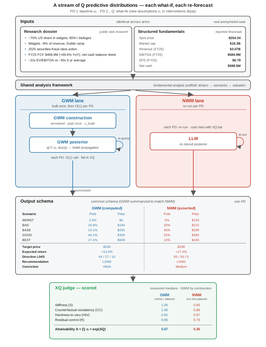
Figure 2: The benchmark task. A case is one stock at a point in time; the target Y is its 12-month forward return, served as a stream of queries that share one model and vary the assumptions u and/or interventions \mathrm{do}(a) (a baseline u_{0}, then re-forecasts and what-ifs). Both arms take identical inputs, follow a shared analysis framework, and report in a common schema; they differ only in the middle—the GWM is built once, then answers each query by O(1) inference at flat cost c_{\mathrm{PD}}, while the NWM re-runs per query at a cost rising with the XQ bar (Eq. (8)). A tool-backed judge scores both on (S,\mathrm{CC},\mathrm{HtV},R); cumulative cost and break-even Q^{\star} are in Figure 4.
3.2 Benchmark results: efficiency and explanation quality
We benchmark the two arms on efficiency and explanation quality, then combine them. Both arms’ efficiency scales with underlying model size, but two things separate them (Figures 3, 4): the GWM’s model is far smaller, and—decisively—a GWM posterior is exact given its evidence, so it delivers its maximal explanation quality (the conditioning-limited ceiling A_{\mathrm{GWM}}) at every predictive distribution regardless of budget and latency constraints, whereas raising a NWM’s XQ demands more thinking tokens, tool calls, and validator iterations, driving cost and latency super-linearly toward an attainability ceiling A_{\mathrm{NWM}} it can only approach.[5] We score quality on the bounded attainability A=\prod_{i}c_{i}=\exp(\mathrm{XQ})\in(0,1] of Eq. (7) and price both arms on two consistent bases—single-generation and incremental per-PD—via the NWM per-PD cost model of Eq. (8) and the break-even of Eq. (12). Appendix C formalizes the two levels a NWM faces—a structural ceiling no budget can clear (Proposition 5, which we generously equate to the GWM’s) and the lower level it attains under finite compute (Proposition 6)—and proves that, because XQ aggregates multiplicatively, the GWM dominates at every finite budget (Corollary 1).
Per-case generation cost and latency.
A Primordia v1 case costs c_{\mathrm{build}}=\$2.35{} (\approx\!408{} s). The NWM arm (Opus 4.8) costs a measured c_{\mathrm{NWM}}=\$1.63{} (\approx\!230{} s) for a standard sourced memo—the median over 20 cases (range $1.21–$1.82)[2026], and 3c_{\mathrm{NWM}} for a full evidence-chain artifact.
Explanation quality of the two arms.
The arms separate on all four XQ axes. The GWM is exact-by-construction on the mechanism (S=\mathrm{CC}=1), with \mathrm{HtV}=0.92 and R=0.95. The narrative arm’s measured components are all well below 1 (S=0.83, \mathrm{CC}=0.88, \mathrm{HtV}=0.67, R=0.73; Table 4)[11]. Because XQ aggregates multiplicatively, these place the NWM’s deployed joint correctness at \prod_{i}c_{i}=0.36 against the GWM’s 0.87—a 2.4\times gap at equal (deployed) cost; a product is capped by its weakest factor. Appendix E reports the same scorecard for the worked case (Table 3).
Cost and latency to reach a quality target.
Pricing both arms on two consistent bases (Figure 3) makes the divergence concrete in dollars and wall-clock. Single generation: a single NWM memo undercuts the GWM build’s cost at a low bar but crosses it at A\approx 0.43 as the output blow-up takes over. Incremental per-PD: the GWM answers each PD at a flat c_{\mathrm{PD}}=\$1.0\times 10^{-6}{} in 0.086 s, while the NWM’s cost and latency climb without bound toward the ceiling—357\times slower on a measured warm re-query (30.9 s) today, and the gap widens as the bar rises. By Proposition 1 this is a statement about prediction quality, not merely its proxy.
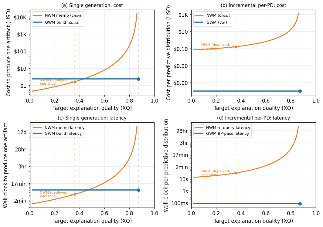
Figure 3: Cost (top) and latency (bottom) to reach a target explanation quality, on two consistent bases. (a)/(c) Single generation: the GWM’s one-time build vs. the NWM’s full sourced memo, each anchored at its measured cost/latency at the deployed attainment. (b)/(d) Incremental per-PD: the GWM’s flat belief-propagation pass vs. the caching-aware NWM re-run of Eq. (8) and its latency analogue. The GWM is flat and sits at the ceiling in every panel; the NWM diverges toward the same (generously shared) ceiling A_{\mathrm{GWM}} (dotted), with the deployed one-shot NWM marked (A\approx 0.36). Target axis: bounded attainment A=\exp(\mathrm{XQ})\in(0,1] (Eq. (7)). Log y-axes; values from Appendix I.
Amortizing the build.
The single-generation parity is an artifact of Q=1. The GWM pays c_{\mathrm{build}} once, then answers every PD at a flat c_{\mathrm{PD}}=\$1.0\times 10^{-6}{} in 0.086 s; the NWM re-runs per PD, even granted its own best-case caching amortization. The break-even Q^{\star}(\mathrm{XQ}) of Eq. (12) (Figure 4) shows the build recouped after \approx\!4{} PDs at a modest target (0.1{}), collapsing to a single PD as the bar rises; above the NWM ceiling (\approx\!0.87{}) no number of runs reaches the target. The same logic applies to wall-clock: the GWM’s slower build is repaid almost immediately once queries stream, since every follow-on PD answers 357\times faster than a warm NWM re-query.[1818181] Appendix E works one real (anonymized) case end-to-end across the PD stream.
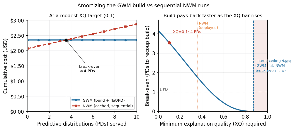
Figure 4: Amortizing the GWM build against sequential, caching-aware NWM runs. Left: at a modest XQ target (0.1{}), cumulative cost crosses at \approx\!4{} PDs—the GWM’s c_{\mathrm{build}} build plus flat c_{\mathrm{PD}}/PD undercuts the NWM, which re-runs (cached) per query. Right: break-even PD count vs. the minimum XQ required; it falls below one PD as the bar rises, and beyond the NWM ceiling (\approx\!0.87{}) no number of runs reaches the target. All values from the shared parameter set (Appendix I).
3.3 Limitations
Our empirical evidence is deliberately scoped, and we are explicit about what is measured versus assumed. The strongest results are direct measurements over the deployed system: per-case build cost (c_{\mathrm{build}}=\$2.35{}/case over 1,184 cases from production logs, \approx\!408 s of wall-clock), the GWM’s flat per-PD inference cost and latency (c_{\mathrm{PD}}\approx\$1.0\times 10^{-6}{}/PD, 0.086 s/PD), and the narrative arm’s per-case generation cost and latency (c_{\mathrm{NWM}}=\$1.63{}, range $1.21–$1.82; \approx\!230 s) and warm re-query latency (30.9 s, the same measured calls that anchor the incremental-PD cost curve). All come from a single domain—equity investing—so the magnitudes should be read as evidence that the architectural gap is real and large, not as a cross-domain performance benchmark; a live track record is out of scope here by design.
The explanation-quality comparison is likewise measured by proxy. We score the narrative arm’s structural components (S, \mathrm{CC}, \mathrm{HtV}) with a tool-backed judge over 20 cases (Section 3.2). The GWM’s own ceiling and its residual-control values R are by-construction (exact posteriors given evidence), not independently audited, and the cost–XQ blow-up exponent is an empirically justified modeling assumption rather than a fit. The XQ\toPQ proxy (Proposition 1) rests on Assumptions 1–2, plausible but unverified for any specific domain.
Finally, one bound is not an artifact of measurement at all: even a perfectly specified, perfectly conditioned GWM is capped by the system’s intrinsic predictability horizon (Section 2.7), which limits the residual-control component R at long lead times. This is a property of the world, not the model, and it bounds both architectures equally.
4 Discussion
4.1 Three usage modes of GWMs
As discussed in Section 1, LLM-powered workflows are increasingly applied to real-world decision tasks. The natural taxonomy is by the driver of the decision loop—who chooses the next action given the GWM’s posterior—which takes three values: a human, an LLM agent, or an algorithm. The first is human-in-the-loop; the latter two are autonomous, distinguished by whether the driver reasons in language or in code (Figure 5).
Mode 1: human-driven (decision-support).
When a GWM informs a human analyst, the GWM’s key value proposition is the trustworthiness justified by XQ (See Prop. 1): a LLM memo can be persuasive while being wrong in ways the analyst cannot audit. An LLM retains its role as a natural-language interface to the GWM’s structured inputs and outputs.
Mode 2: LLM-driven (neurosymbolic agent).
We foresee deployments pairing the GWM with an autonomous LLM agent, where the GWM is the verified predictive core that lends the agent stiffness and reliability: the LLM explores, frames, and explains, while the GWM computes the posterior, thus implementing the neurosymbolic pattern proposed in Garcez (2025). The instructive contrast is with GraphRAG (Edge et al., 2024), which augments the LLM with a static knowledge graph: it raises assumption consistency but returns text, not a posterior under an explicit mechanism, so it gains neither grounding nor proper Bayesian updating. The analogy that does work is the coding harness—just as agents increasingly call deterministic, verified code rather than re-deriving it, a decision agent should call a verified GWM rather than re-asserting probabilities. In the RAIL design space of Chiatti et al. (2026), this places the GWM at the demanding corner of every axis at once—verified-by-design assurances, structured-symbolic interfacing, and knowledge-guided learning—with the LLM supplying the neural, exploratory half; it is precisely this combination, rather than any single axis, that the narrative baselines forgo.
Mode 3: algorithm-driven (MPC / active inference).
When a GWM drives a control loop with no language model in the decision path—rebalancing a position, dispatching capital—predictions must be produced on a fixed cadence and support counterfactual rollouts for planning. This is model-predictive control (MPC), and in the probabilistic setting, active inference (Friston et al., 2017): the agent selects actions minimizing a expected free energy functional under \mathcal{M}.
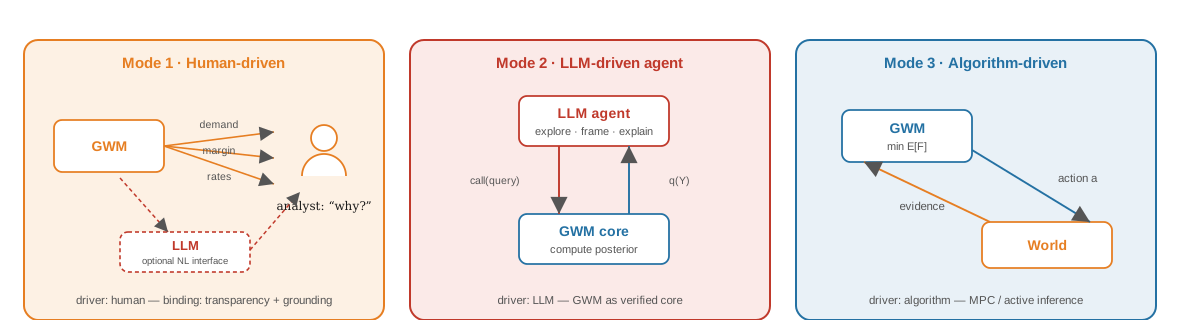
Figure 5: The three usage modes, organized by the driver of the decision loop. Mode 1 (human-driven) feeds a named pathway decomposition to a human analyst; an LLM optionally mediates as a natural-language interface. Mode 2 (LLM-driven) makes the GWM the verified core of a neurosymbolic agent, with the LLM as its language interface. Mode 3 (algorithm-driven) closes a control loop—the GWM powers an action-selection module and the world returns evidence.
4.2 An illustrative look at cost and capability
Figure 6 situates the GWM against the general-purpose LLM cost/capability frontier of July 2026. The point is deliberately illustrative—the GWM does not carry an Intelligence Index score, since it is not a general-purpose model—but the qualitative claim is precise: the GWM is not another point competing on this frontier, it is a domain-specific capability that a Mode-2 agent calls on relevant tasks, the same way it calls a verified code tool, thus obtaining strict improvements along both cost and capability axes.[2026]
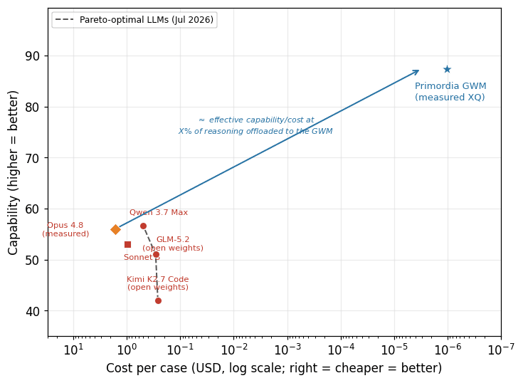
Figure 6: The dashed curve estimates the general-purpose LLM cost/capability frontier as of July 2026 (Artificial Analysis Intelligence Index; Artificial Analysis, 2026b, a; FelloAI, 2026; The Decoder, 2026; Artificial Analysis, 2026c). Every LLM’s published price is converted to an estimated USD/case by anchoring on our own measured Opus 4.8 arm (c_{\mathrm{NWM}}=\$1.63{}; Section 3) and scaling by output-token price. The GWM sits off this frontier entirely; the arrow marks Mode 2 composition—an agent on the frontier offloading its prediction subtask to the GWM—not substitution.
4.3 Why a GWM is capital
A GWM is reusable capital: built and verified once for a task class, then applied to many instances at near-zero marginal cost (the amortization of Section 3.2). This is what makes “call a verified model” the rational default over “re-derive each time”—what we call the returns to crystallization. The intuition is that a valid solution to a high-stakes task must satisfy a product of constraints at once, so the cost of finding one afresh grows exponentially in task complexity, whereas reusing a verified model costs only an O(1) grounding step. The resulting leverage is large and—decisively—is dominated by failure avoidance: the value destroyed when an unverified search silently fails and propagates downstream, a term that does not shrink as token prices fall (we make this quantitative in Appendix B). Hence a rational principal does not re-derive a grounded model per instance; it calls a verified one, exactly as agentic coding increasingly calls verified library code rather than re-synthesizing it—and because a GWM’s reuse cost is the grounding inference itself, climbing the groundedness ladder and earning this leverage are the same act.
4.4 Generalization and scope
Little in this paper is specific to finance. Any domain requiring structural causal prediction—supply-chain risk, epidemiology, grid planning, macroeconomic policy—has the same groundedness axis and the same contrast between a verified posterior and a narrated one. The GWM structure transfers directly; only the latents and the evidence change. That said, any given GWM only produces predictions within its domain, by construction; the definition of a domain is arbitrary and can extend well beyond typical discipline walls, but we do not foresee the construction of a single GWM capable of answering arbitrary queries on any domain in the same sense as LLMs can; at least in the short term, combining domain-specific GWMs with an orchestrator LLM as in Modes 1 and 2 of Section 4.1 appears to be a highly valuable pragmatic compromise.
For simplicity, this paper treats predictions for different cases as siloed, independent contexts. However, a decision-maker typically must make decisions that are coupled across cases—for instance, stocks in a portfolio are typically causally correlated. A GWM can naturally be structured to represent such real-world couplings, producing joint posteriors over an effectively unlimited universe. Doing so reveals an even more striking advantage against NWMs, which must maintain coherence across cases using LLM attention mechanisms, at superlinear cost and without any structural guarantees. We will expand on this significantly in a follow-up paper (Kaufmann et al., 2026).
5 Conclusion
Real-world, high-stakes decision-making demands a causal posterior, which must be produced by a grounded world model. An LLM can narrate or improvise predictions, but it cannot reliably be a posterior: its non-Bayesian updating does not keep a prediction proper as evidence arrives (Proposition 3), and scaling the model does not help—the prior probability that its circuit implements exact conditioning only decreases with size (Corollary 2). Continual learning does not rescue it either—a gradient step is no more Bayes’ rule than a context update (Corollary 3). The question is not whether a language model can emit a number, but whether that number can be grounded, and at what cost.
As seen in Section 3, our v1 GWM answers each query by inference on a model orders of magnitude smaller than an LLM, providing grounded predictions at negligible marginal cost, and amortizing its build within a handful of predictive distributions (Section 3.2). Meanwhile, an LLM either faces diverging cost or must replicate an ad hoc GWM per query. Further, a GWM’s explanation quality dominates a narrative model’s at every budget (Section 3.2)—a structural gap that scaling the language model makes less likely to close, not more (Corollary 1). The comparison is measured over a public benchmark sample and released for replication (Section 3.1); v1 itself is deployed across \sim\!12{,}000 equities.
The implication is architectural and wide-ranging. Because a verified GWM is reusable capital (Section 4.3), the efficient deployment of agentic AI points toward a shared library of composable world models rather than per-query renarration: a division of labor in which the language model frames and explains and the GWM computes the posterior. This is also how automation’s efficiency can be reconciled with the accountability it displaces (Section 1): the LLM-powered workflows replacing risk-aware human judgment can answer the right questions correctly only by offloading the critical computations to a “known-good” model—exactly as a builder offloads physical computation to a CAD engine.
The economic benefits of offloading are significant. Beyond the first-order effect of strictly improving agent performance along both cost and quality axes by replacing slow, opaque, autoregressive narrative with structured prediction (Section 4.2), offloading has significant multiplier effects: by providing known-quality, uncertainty-aware predictions in one shot, it prevents sharply compounding verification and rework costs arising from error and false confidence (Meyerson et al., 2025; Ro et al., 2025); mitigates the costs and complexity associated with managing long LLM context (Liu et al., 2024; Du et al., 2025); and enables risk-mitigation policies that are deterministic, verifiable and demonstrably aligned with organization policies (Walters et al., 2025a). Hence, given the ubiquitous need for structural causal prediction in the sort of day-to-day knowledge work being automated by LLMs, we suggest that a significant fraction of a typical business LLM agent’s token stream will be offloaded to GWMs as they become available for more domains, thus making business AI more economical, safe, and trustworthy.
Acknowledgments
We thank Dimitrije Marković, Thomas Kopinski, Michael Walters, Felix Neubürger and Artur d’Avila Garcez for valuable discussions and feedback.
Appendix A Instantiation of Numerical Weather Prediction as a GWM
GWM element | Numerical weather prediction counterpart |
|---|---|
Explicit causal mechanism | Discretized Navier–Stokes |
Grounding map | Data assimilation: 4D-Var / ensemble Kalman filter over millions of daily observations (Kalnay, 2003). |
Predictive distribution (PD) | Ensemble forecast: perturbed initial conditions |
Verified correctness / invariants | Conservation of mass, energy, and momentum enforced by the integrator. |
Predictability horizon | Lyapunov limit on forecast lead time (Lorenz, 1963). |
Table 1: Numerical weather prediction realizes the GWM contract element by element—the most mature deployed grounded world model.
Appendix B The Returns to Crystallization
This appendix gives the formal return structure behind the reusable capital argument of Section 4.3. Searching for a fresh, valid solution to a task of complexity \kappa is expensive because a non-trivial objective is a product of constraints that must all hold at once; valid solutions occupy a sparse island whose measure decays geometrically in the number of binding constraints m(\kappa). The expected search cost thus scales like \bar{q}^{-m(\kappa)}\,\xi(\kappa) (with \bar{q}<1 the per-constraint pass rate and \xi\geq 1 a backtracking overhead), while reusing a verified model costs only an instance-adaptation factor \rho(\kappa)=O(1)—for a GWM, the grounding inference of (13) that ties parameters to this instance’s evidence. Their ratio is the crystallization leverage
\Lambda(\kappa)\;=\;\frac{\text{search cost}}{\text{reuse cost}}\;=\;\frac{ \bar{q}^{-m(\kappa)}\,\xi(\kappa)}{\rho(\kappa)},
(2)
which grows exponentially in \kappa, since the numerator does and \rho is bounded. Calibrated to current frontier per-step reliability, \Lambda\approx 160\times for a four-hour task and >6{,}000\times for a full workday task.
Token leverage is only half the incentive. Writing V(\kappa) for task value, P_{\text{succ}}(\kappa) for the probability that an unverified search succeeds, and \delta(\kappa)\geq 1 for the damage multiplier when it fails and the bad output propagates downstream, the per-invocation gain from using a verified model decomposes into two additive terms:
\Delta(\kappa)\;=\;\underbrace{V(\kappa)\,(1-P_{\text{succ}})\,(1+\delta( \kappa))}_{\text{failure avoidance}}\;+\;\underbrace{T_{\text{reuse}}(\kappa) \,(\Lambda(\kappa)-1)}_{\text{token savings}}.
(3)
The token-savings term shrinks as inference prices fall; the failure-avoidance term does not. For the high-stakes, many-constraint tasks that dominate the high-\kappa regime it is the binding incentive—at \kappa=10 it already reaches \approx 3.96\,V per invocation—and it persists even as token costs approach zero.
Appendix C Explanation-Quality Components and Heuristic Parameter Derivations
This appendix gives formal definitions for the four components of \mathrm{XQ} (Definition 7).
Let q be a PD produced by a computation with named structural inputs \theta=(\theta_{1},\dots,\theta_{m}), a set of invariants \mathcal{I} (accounting identities, sign and monotonicity constraints), and—for sampling-based WMs—a Monte-Carlo budget yielding standard error \mathrm{se}(q) on a target summary functional T(q) with natural scale \tau. Fix a battery \mathcal{A} of intervention queries.
Definition 8 (Rationale stiffness).
Let \varepsilon_{j}=\partial\log T(q)/\partial\log\theta_{j} be the elasticity of T to input \theta_{j}, and B_{j} the mechanism-implied admissible band for that elasticity. Then
S(q)\;=\;\frac{1}{m}\sum_{j=1}^{m}\mathbf{1}\!\left[\varepsilon_{j}\in B_{j} \right]\;\in\;[0,1],
(4)
the fraction of inputs that are not free knobs (responses bounded and mechanism-consistent).
Definition 9 (Counterfactual consistency).
\mathrm{CC}(q)\;=\;\frac{1}{|\mathcal{A}|}\sum_{a\in\mathcal{A}}\mathbf{1}\! \left[\,q(\cdot\mid\mathrm{do}(a))\text{ satisfies }\mathcal{I}\text{ and the do-calculus identities}\,\right]\;\in\;[0,1].
(5)
Definition 10 (Hardness-to-vary).
For an alternative outcome y^{\prime}, let q^{\prime} be the nearest model (minimal structural edit) that fits y^{\prime} without violating \mathcal{I}, and \delta(y^{\prime})=d(q,q^{\prime})/d_{\max}\in[0,1] the normalized forced change. Then \mathrm{HtV}(q)=\mathbb{E}_{y^{\prime}}[\delta(y^{\prime})]: a high value means the explanation cannot be cheaply twisted to fit a different outcome (Deutsch, 2011).
Definition 11 (Residual-noise control).
R(q)=1-U(q)\in[0,1], where U(q) is the residual uncertainty about the true posterior left by the computation that produced q; R=1 in the exact-inference limit. For a sampling WM with Monte-Carlo standard error \mathrm{se}(q) and tolerance \tau, U=\min\!\big{(}1,\mathrm{se}(q)/\tau\big{)}, which vanishes in the large-sample limit. A single narrative emission instead asserts one scenario distribution while its qualitative rationale pins only a set B of distributions on the K-scenario probability simplex \Delta^{K-1}; the residual uncertainty is then the linear extent of that set, U=\big{(}\mathrm{vol}(B)/\mathrm{vol}(\Delta^{K-1})\big{)}^{1/(K-1)}, so R=1-\big{(}\mathrm{vol}(B)/\mathrm{vol}(\Delta^{K-1})\big{)}^{1/(K-1)} (estimated in Appendix C).
The four components are independent correctness probabilities, so the joint correctness of q is their product and explanation quality is the corresponding log-probability:
\mathrm{XQ}(q)\;=\;\sum_{i}\log c_{i}\;=\;\log S(q)+\log\mathrm{CC}(q)+\log \mathrm{HtV}(q)+\log R(q)\;\leq\;0,
(6)
measured in nats, on the same scale as \mathrm{PQ}=-D_{\mathrm{KL}}. Near the ideal, -\mathrm{XQ}=\sum_{i}(-\log c_{i})\approx\sum_{i}(1-c_{i}), which recovers to first order the linear KL bound used in the proof of Proposition 1; the log form is its all-orders extension, and unlike an arithmetic mean it admits no cross-component compensation—a single weak axis caps the whole. For figures and quality targets we use the bounded attainment
A(q)\;=\;\exp\!\big{(}\mathrm{XQ}(q)\big{)}\;=\;S\,\mathrm{CC}\,\mathrm{HtV}\, R\;\in\;(0,1],
(7)
the joint-correctness probability of the four axes—a strictly monotone transform of \mathrm{XQ} (indeed \mathrm{XQ}=\log A), so every ceiling and ordering statement transfers between the two, and a ratio of two A’s is exactly the exponential of their \mathrm{XQ} difference.
A note on scale, to avoid a common confusion. \mathrm{XQ}\in(-\infty,0] itself is the log-scale quantity Proposition 1 lower-bounds \mathrm{PQ}=-D_{\mathrm{KL}}(p^{\star}\|q) by, and—exactly as intuition suggests—it increases toward (though it need not reach) 0 as q becomes a better explanation, mirroring \mathrm{PQ}\to 0 as q\to p^{\star}; this is not in tension with attainment being bounded. What lives on the familiar [0,1] scale is not \mathrm{XQ} but A=\exp(\mathrm{XQ})\in(0,1]. Because the two are a strictly monotone transform of each other, we use them interchangeably in prose below for readability—so wherever the text speaks of “raising XQ,” an “XQ target,” or an “XQ ceiling” expressed as a number in (0,1), it denotes this bounded attainment A, not the log-scale \mathrm{XQ} of Eq. (6), which is what is actually being plotted or bounded in Sections 3.2 and the propositions below.
Operational estimators of the components
The definitions above are population quantities over a battery \mathcal{A} and an invariant set \mathcal{I}; we now state how each is estimated on the narrative-arm memos (the measurement of Section 3.1), so the reported scores map transparently onto Definitions 8–11. A tool-backed judge agent (also Claude Opus 4.8) reads each memo equipped with a sandboxed arithmetic evaluator and a numerical closeness check; it may verify a number only by calling a tool, so the structural scores are tool-checked rather than asserted, and the full call log is persisted per case for audit.
• Stiffness S (Def. 8). The fraction of headline numbers (target price, expected return, direction probabilities, the weighted scenario value, each multiple-to-price bridge) that are reconstructible from other stated inputs in the memo. A number that no stated inputs reproduce is a free knob—an unconstrained elasticity direction, the discrete analogue of \varepsilon_{j}\notin B_{j}.
• Counterfactual consistency \mathrm{CC} (Def. 9). Estimated in two steps and combined as \mathrm{CC}=\min(\mathrm{CC}_{\mathrm{stat}},\mathrm{CC}_{\mathrm{int}}), so the weaker step caps the score. Step 1 (static internal consistency): the battery that probabilities sum to one; the stated target equals the probability-weighted scenario prices; expected return = target/spot -1; the direction buckets match the scenario upsides; scenario prices are monotone in severity; and the recommendation’s sign lies in the stated return band—each an instance of “q satisfies \mathcal{I},” checked with the tools. This step certifies only that the memo is self-consistent, not that it answers \mathrm{do}(a) correctly. Step 2 (interventional re-query): to test the do-calculus clause of Definition 9 directly, the judge poses at least five off-grid interventions \mathrm{do}(a)—probes whose correct answer is neither any tabulated scenario price nor a convex re-weighting of them, spanning between-scenario, compound, fixed-input, and mechanism-inversion families—and re-queries the same NWM under each, holding its stated thesis and mechanism fixed. Each re-forecast is scored continuously in [0,1] for whether it tracks the memo’s own stated mechanism in both direction and magnitude (no external oracle), and \mathrm{CC}_{\mathrm{int}} is their mean.
• Hardness-to-vary \mathrm{HtV} (Def. 10). The one component scored as a direct judgment: the minimal structural edit needed to make the rationale fit the opposite recommendation without breaking an invariant, in [0,1].
• Residual-noise control R (Def. 11). Measured per memo. The judge brackets each of the K scenario probabilities by a band [\ell_{k},u_{k}] that the narrative defensibly supports; a deterministic tool computes the fraction f=\mathrm{vol}(B)/\mathrm{vol}(\Delta^{K-1}) of the simplex compatible with those bands (by uniform-simplex sampling), and R=1-f^{1/(K-1)}. A tightly argued distribution gives small f and high R; a vague one gives R\to 0. The GWM’s large-sample R is taken as the NWM’s generous ceiling (reachable only by MC-averaging many emissions), not as its deployed value.
Appendix D The Sampling Budget: Latency vs Residual Monte-Carlo Error
Every GWM headline (target price, direction probabilities, scenario mix) is a functional of n_{\mathrm{samples}} Monte-Carlo draws, so the sample budget trades latency against the residual noise that enters the residual-noise control R(q)=1-\min(1,\mathrm{se}(q)/\tau) of Definition 11. We fix n_{\mathrm{samples}}=10{,}000 throughout; this appendix justifies that choice. Sweeping by powers of ten over the cost-benchmark cases of Appendix F (warm median wall-clock; standard error of T(q)=\mathbb{E}[\text{upside}] estimated as \mathrm{se}(q)=\hat{\sigma}_{\text{upside}}/\sqrt{n_{\mathrm{samples}}}), Figure 7 plots the tradeoff.
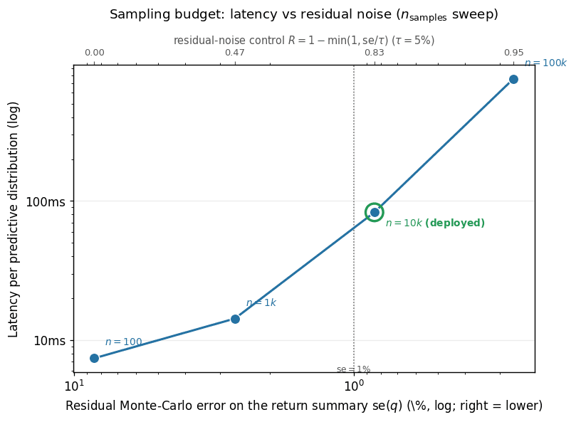
Figure 7: Choosing the sampling budget: latency vs residual noise. Latency per predictive distribution (log, vertical) against the residual Monte-Carlo standard error on the return summary (log, horizontal; right = lower error = better), swept over powers of ten and aggregated as the median over recent deployed v1 cases. The residual falls as the textbook n^{-1/2} (each decade cuts it \approx 3.2\times), while latency is flat below a per-call overhead floor and then rises roughly linearly—so the curve’s geometric elbow is near n{=}1\text{k}, not at the deployed budget. We nonetheless deploy n{=}10\text{k} (circled) for sufficiency, not because it is the elbow: it is the smallest budget whose residual clears the decision-relevant \mathrm{se}\!\approx\!1\ band (dotted; R\!\approx\!0.83 at \tau{=}5\) while latency is still sub-100ms. The elbow at 1\text{k} is too noisy (\mathrm{se}\!\approx\!2.7\, R\!\approx\!0.47—enough to flip a direction call), and the next decade to 100\text{k} pays \approx 9\times the latency for a further \sqrt{10} residual reduction that no longer moves a decision. The top axis reads the same residual as the bounded residual-noise control R=1-\min(1,\mathrm{se}/\tau) (Def. 11).
Two regimes bracket the choice: below \sim\!10^{3} samples a fixed per-call overhead floors the latency while the residual balloons, and above \sim\!10^{4} the sampling loop dominates, so each further decade costs a near-full decade of latency for only a \sqrt{10} residual gain. The 10{,}000-sample budget clears the floor and drives R into saturation at sub-second latency; because the residual scales as n^{-1/2}, only the absolute latency floor (hardware) moves with the case mix, not the choice itself.
Appendix E A Worked Example: GWM vs NWM on One Case
This appendix grounds the protocol of Section 3.1 in one real case from the sample—anonymized as ACME, spot $254.34—showing both the single-PD quality contrast and the cost of a stream of PDs. All numbers are taken from the released artifacts: the NWM memo and its tool-checked judge log, and the GWM’s evaluated posterior.
One PD: the quality contrast
Both arms received the same dossier and fundamentals and emit the same schema. Table 2 places the two outputs side by side.
NWM (asserted) | GWM (computed) | |||||
Scenario | Prob | Price | Upside | Prob | Price | Return |
WORST | 5% | $150 |
| 2.6% | $0 |
|
BAD | 20% | $215 |
| 18.8% | $184.0 |
|
BASE | 40% | $298 |
| 15.1% | $255.0 |
|
GOOD | 25% | $360 |
| 46.1% | $368.7 |
|
BEST | 10% | $430 |
| 17.4% | $608.5 |
|
Target price | $298 | $289.7 | ||||
Expected return |
|
| ||||
Direction L/H/S | 65 / 30 / 5 (table implies 75 / 20 / 5) | 63.5 / 26.8 / 9.7 | ||||
Recommendation | LONG | LONG | ||||
Conviction | Medium | HIGH | ||||
Table 2: ACME, side by side: asserted vs computed (spot $254.34). Red = asserted by the model; blue = computed from the posterior (read off the same Monte-Carlo samples). The NWM’s direction probabilities (65/30/5) are a free knob that contradicts its own scenario table, which implies 75/20/5; the GWM’s (63.5/26.8/9.7) are \Pr(\text{upside}>\text{hurdle}) over the scenario samples and so cannot disagree with the table. The GWM target is the probability-weighted geometric-mean certainty-equivalent (vs the NWM’s arithmetic weighted price), and its WORST bucket is a sub--78.8\ wipeout tail.
What the judge finds.
The tool-backed judge (Appendix C) reconstructs the NWM’s headline numbers with its calculator: the target reconstructs as the probability-weighted price (\sum_{i}p_{i}\,P_{i}=302.7\approx 298, within 2\), expected return as 298/254.34-1=+17.2\, and each scenario upside as P_{i}/254.34-1—all pass. One number does not reconstruct: the asserted direction probabilities 65/30/5 contradict the scenario table, which implies 40{+}25{+}10=75\ LONG, 20\ HOLD, 5\ SHORT. This single free knob fails one of nine static consistency checks (\mathrm{CC}_{\mathrm{stat}}=8/9=0.889) and one of seven stiffness checks (S=6/7=0.857). Probing further, the judge re-queried the same NWM under five off-grid interventions—a between-scenario multiple compression, a buyback that accretes EPS, a compound revenue/margin shift, an interpolated revenue/margin/multiple triple, and a breakeven-multiple inversion, none answerable from the scenario table—and every re-forecast tracked the memo’s own EPS\timesmultiple bridge in direction and magnitude (\mathrm{CC}_{\mathrm{int}}=1.0), so \mathrm{CC}=\min(0.889,1.0)=0.889. Hardness-to-vary is judged 0.62 (the soft scenario probabilities and a reversible narrative can be re-spun for a bear case without breaking the arithmetic). Residual control is measured from the probability bands the narrative supports: only f=0.8\ of the five-scenario simplex is compatible, giving R=1-f^{1/4}=0.705—high, but below the GWM’s large-sample 0.95.
The GWM has no such knob to break. Its scenario probabilities sum to one, each scenario upside equals P_{i}/\text{spot}-1, prices are monotone in severity, and—crucially—its direction probabilities are not asserted but read off the same posterior samples as the scenarios, so they cannot disagree with the table. Stiffness and counterfactual consistency are therefore 1 by construction (Table 4); the residual gap to a perfect explanation is bounded misspecification (\mathrm{HtV}=0.92) and Monte-Carlo residual (R=0.95), not a free parameter. Table 3 collects the scores.
Component | NWM (ACME) | NWM (median) | GWM |
|---|---|---|---|
Stiffness |
|
|
|
Counterfactual consistency |
|
|
|
Hardness-to-vary |
|
|
|
Residual control |
|
|
|
Attainment | — |
|
|
Table 3: Explanation-quality scorecard for the worked case. ACME’s measured (S,\mathrm{CC},\mathrm{HtV},R) are near the sample medians, yet still bounded well away from the GWM’s S=\mathrm{CC}=1. Because XQ aggregates multiplicatively (Eq. (6)), the NWM’s joint correctness trails the GWM by 2.4\times.
Across the stream.
Table 3 is the Q{=}1 slice, which most flatters the NWM. ACME is in fact queried repeatedly—each what-if and re-forecast is another PD—so its per-case economics are those of Sections 3.2–3.2: ACME’s GWM build is paid once, and every follow-on PD, including the \mathrm{do}(a) battery (re-rating the exit multiple, shifting demand, flipping ValuationReRates), is a flat c_{\mathrm{PD}} call that preserves the invariants above (\mathrm{CC}{\to}1). A one-shot NWM run costs up to $1.82 and buys no reusable posterior (only a KV cache of the run’s input and output tokens), so every additional PD is another run at a cost that climbs with the XQ bar. The crossover and ceilings are exactly those of Figure 4.
Appendix F Cost-Model Details
This appendix states the narrative arm’s per-PD cost model used in Section 3, the assumptions behind it, and the resulting blow-up claim; the proof is deferred to Appendix G.
Setup
Writing the cached-context re-read as T_{\mathrm{cache}}\,p_{\mathrm{cache}} and the per-PD output as n\,T_{\mathrm{out}}\,p_{\mathrm{out}} scaled by a quality-dependent blow-up factor,
c_{\mathrm{NWM}}(\mathrm{XQ})\;=\;\underbrace{T_{\mathrm{cache}}\,p_{\mathrm{ cache}}}_{\text{cached re-read}}\;+\;\underbrace{n\,T_{\mathrm{out}}\,p_{ \mathrm{out}}\left(\frac{A_{\mathrm{NWM}}}{A_{\mathrm{NWM}}-\mathrm{XQ}}\right )^{\eta}}_{\text{output (diverges at the ceiling }A_{\mathrm{NWM}})},
(8)
where A_{\mathrm{NWM}} is the NWM’s structural ceiling (Proposition 5), T_{\mathrm{out}} the tokens to narrate one PD, \eta>0 the cost–quality blow-up exponent, and n\geq 1 the number of emissions MC-averaged into one PD.
After Eq. (8), the ceiling A_{\mathrm{NWM}} is budget-invariant—a structural supremum no spending can exceed (Proposition 5), and for quantification we generously set it equal to the GWM’s, A_{\mathrm{NWM}}=A_{\mathrm{GWM}}—so it fixes the pole location. What a larger budget does buy is a higher achieved XQ: unstructured validator iteration certifies progressively more of the checkable invariants (the stiffness reconstructions, the static-CC consistency checks, and the HtV-hardening edits), pushing the achieved attainment up toward A_{\mathrm{NWM}} at a per-PD cost that diverges as \mathrm{XQ}\uparrow A_{\mathrm{NWM}}. Residual control is improved not by validator iteration but by MC-averaging emissions (the factor n above); we grant its large-sample value only as the ceiling, while the one-shot deployed memos attain a measured R=0.73<0.95 (Appendix C). The numerical value of \eta is calibrated (Appendix I); the claim below identifies it.
Coverage and the cost of adversarial certification
Throughout, the XQ target is set by an ideal adversarial validator that maintains an unbounded battery of checkable invariants—the interventional queries of Definition 9 together with the structural reconstructions of Definitions 8 and 10—and certifies the NWM’s predictive only when it jointly passes a finite subset of size \nu. We derive the two ingredients of the blow-up (coverage and cost) rather than assume them.
Lemma 1 (Saturating coverage).
Let x<x_{c} (x_{c}=A_{\mathrm{NWM}}, Proposition 5) be the attainment reached when the predictive jointly passes \nu invariants drawn from the battery, and write the residual incorrectness r=1-x/x_{c}\in(0,1). Because XQ aggregates multiplicatively (Eq. (6)), certifying one further invariant removes a fraction of r that is bounded away from 0, so in the continuum limit
\frac{dx}{d\nu}=\lambda\,(x_{c}-x),\qquad\lambda>0.
(9)
Proof.
Joint correctness is the product \prod_{i}c_{i} of per-invariant correctness events (Eq. (6)), so the residual r=1-x/x_{c} is the surviving share of error. An adversary never spends a query on a check already implied by the passed set, and draws invariants of comparable difficulty; hence certifying the (\nu{+}1)-th invariant multiplies the surviving error by a stationary factor 1-\beta with \beta\in(\beta_{0},1), \beta_{0}>0. Thus r(\nu{+}1)=(1-\beta)\,r(\nu), i.e. dr/d\nu=-\lambda r with \lambda=-\ln(1-\beta)>0; substituting r=1-x/x_{c} gives (9). ∎
Lemma 2 (Adversarial certification is geometrically hard for a mechanism-free model).
A narrative WM certifies invariants only by local edits to its state—appended context tokens, retrieved snippets, or gradient steps—none of which is the Bayesian conditioning operator B_{e} (Proposition 3), and none of which supplies the unified internal mechanism that would satisfy the invariants jointly (Appendix H). Then there is a per-invariant pass rate \bar{q}<1 such that the expected number of O(1) refinement passes to jointly certify \nu invariants is bounded below by the crystallization law of Appendix B,
k(\nu)\;\geq\;\bar{q}^{-\nu}.
(10)
Proof.
We mirror the measure argument of Proposition 3. (i) Each pass is non-generic. The edit that fixes a freshly drawn invariant maps the state to a new predictive which, by Proposition 3(i), coincides with the Bayes-conditioned target only on a measure-zero subset of states; passing the invariant is therefore a non-generic event of probability at most some \bar{q}<1. This bound is uniform over the battery: were it not—were some sequence of edits to drive the joint pass rate to 1 across the unbounded battery—then by Richens and Everitt (2024) the NWM would have to embed an approximate causal model and route each intervention to it as a conditioning operation, i.e. its internal state would always implement a GWM even as autoregressive decoding perturbs it. By the non-generic-circuit measure of Proposition 3 (the subset of |L|-parameter circuits implementing exact conditioning has prior measure decreasing in |L| and K) this event does not occur for a mechanism-free L, so \bar{q}<1 strictly. (ii) Constraints do not co-crystallize. Because no shared mechanism enforces the invariants jointly, the edit that passes invariant \nu{+}1 is uncorrelated with those that passed 1,\dots,\nu and regresses each with positive probability; the \nu pass-events are thus no better than independent, and the joint-pass (all-certified) set has measure at most \bar{q}^{\nu}. This is exactly the sparse-island structure of Appendix B with m=\nu binding constraints, whose expected search cost is \bar{q}^{-m}; hence k(\nu)\geq\bar{q}^{-\nu}. ∎
Claim
Proposition 4 (NWM cost blow-up).
Combining Lemmas 1 and 2, the NWM per-PD cost follows the output term of Eq. (8) with the exponent identified:
C(x)\;\propto\;\bar{q}^{-\nu(x)}\;=\;\Big{(}\frac{x_{c}}{x_{c}-x}\Big{)}^{\eta },\qquad\eta\;=\;\frac{\ln(1/\bar{q})}{\lambda}\;>\;0.
(11)
Moreover the pole at x_{c} is impassable for a categorical, not a budgetary, reason: crossing it requires \mathrm{CC}\to 1, which by Richens and Everitt (2024) entails an (approximate) causal mechanism—becoming a GWM—unavailable to a mechanism-free model confined to its function class.
Remark (residual sub-lever). When the predictive is estimated from n sampled emissions rather than emitted wholesale, reducing the Monte-Carlo residual adds a second cost scaling as (1-R)^{-2} (error \varepsilon\propto n^{-1/2}, cost linear in n)—the \eta{=}2 special case—which only reinforces the divergence. Proposition 4 thus establishes the output term of Eq. (8) and pins \eta to interpretable quantities; the cost diverges at the structural ceiling, which we generously set equal to the GWM’s (the true ceiling lying strictly below).
Pricing bases and break-even
Both arms are priced on two consistent bases (Figure 3). On the single-generation basis the GWM pays a one-time build c_{\mathrm{build}} (yielding a reusable posterior) against the NWM’s first run c^{\uparrow}_{\mathrm{NWM}}+c_{\mathrm{NWM}}(\mathrm{XQ}); on the incremental per-PD basis the GWM pays a flat belief-propagation pass c_{\mathrm{PD}} against c_{\mathrm{NWM}}(\mathrm{XQ}) per query. Cumulative cost after Q predictive distributions is C_{\mathrm{GWM}}(Q)=c_{\mathrm{build}}+Q\,c_{\mathrm{PD}} versus C_{\mathrm{NWM}}(Q)=c^{\uparrow}_{\mathrm{NWM}}+Q\,c_{\mathrm{NWM}}(\mathrm{XQ}), so the build is recovered after
Q^{\star}(\mathrm{XQ})\;=\;\frac{c_{\mathrm{build}}-c^{\uparrow}_{\mathrm{NWM} }}{c_{\mathrm{NWM}}(\mathrm{XQ})-c_{\mathrm{PD}}}
(12)
predictive distributions (Figure 4); Q^{\star} falls below one as the quality bar rises and is undefined once \mathrm{XQ} exceeds the NWM ceiling, where the NWM cannot reach the target at any budget.
Appendix G Proofs
Throughout, q_{E} denotes a GWM’s posterior predictive for Y after conditioning on evidence E (Eq. (1)), and p^{\star} the reference of Definition 6. Grounding is the following conjugate Beta–Bernoulli update:
p(h\mid E)=\mathrm{Beta}\!\left(\alpha_{h},\beta_{h}\right),\qquad\alpha_{h}=1 +\!\!\sum_{e\in E^{+}_{h}}\!\!w_{e},\quad\beta_{h}=1+\!\!\sum_{e\in E^{-}_{h}} \!\!w_{e},
(13)
where w_{e} is the trust weight of source e and E^{+}_{h},E^{-}_{h} are supporting and refuting evidence Hence, at the level of each evidentiary hypothesis the model is well-specified and the update is exact Bayesian conditioning.
The results below use two assumptions, stated here (the counterfactual battery \mathcal{A} and invariant set \mathcal{I} are formalized in Appendix C).
Assumption 1 (Representative checks).
The finite battery \mathcal{A} of counterfactual queries and the invariant set \mathcal{I} are representative of the query/outcome distribution of interest, so that certifying them bounds the error on untested queries up to an O(\epsilon) remainder.
Assumption 2 (Bounded misspecification).
The GWM is not grossly misspecified: p^{\star} (or its best computable approximation, in the M-open case) lies within the support of the model class entertained by g.[2021]
Empirical support. These realizability conditions are supported by confidential quantitative and qualitative data from forward-testing and daily system usage (internally since December 2025, publicly live since February 2026). A follow-up paper will provide public evidence that the class entertained by g contains a sufficiently accurate, recoverable causal model of the target domain, i.e. that realizability binds in practice and not merely in principle.
Lemma 3 (Prequential information bound).
Let evidence E_{t}=\{e_{1},\dots,e_{t}\} accrue under p^{\star}, and suppose the prior assigns mass \pi^{\star}>0 to the hypothesis realized by p^{\star} (Assumption 2). Then the Bayes predictive losses satisfy
\sum_{t\geq 1}\mathbb{E}_{p^{\star}}\,D_{\mathrm{KL}}\!\big{(}p^{\star}(\cdot \mid E_{t-1})\,\|\,q_{E_{t-1}}\big{)}\;\leq\;-\log\pi^{\star}\;<\;\infty.
(14)
In particular the expected per-step divergence is summable, hence \to 0, and cannot persistently increase.
Proof.
The cumulative log-loss of the Bayes mixture predictor telescopes to -\log of the marginal likelihood of the data, and the marginal likelihood is bounded below by \pi^{\star} times the truth’s likelihood (retain only the true component of the mixture). Taking expectations under p^{\star} and applying the chain rule of relative entropy yields (14); this is the standard prequential/MDL redundancy bound for Bayesian mixtures (Hoeting et al., 1999; Solomonoff, 1964). Summability of the non-negative terms forces them to 0. ∎
Proof of Proposition 2 (Bayesian quality guarantee)
Proof.
Finiteness. By Assumption 2, p^{\star} (or its best computable approximation, in the M-open case) lies in the support of the class entertained by g, so q_{E} is absolutely continuous with respect to p^{\star} on the relevant support and D_{\mathrm{KL}}(p^{\star}\|q_{E})<\infty.
Monotonicity. For the conjugate update (13), the posterior predictive is the Bayes-optimal predictor under log-loss. By Lemma 3 the expected divergence is summable and cannot persistently increase; for a single well-specified conjugate family it is monotone non-increasing at each step, since absorbing e only sharpens \mathrm{Beta}(\alpha_{h},\beta_{h}) toward the realized frequency. Hence \mathbb{E}\,D_{\mathrm{KL}}(p^{\star}\|q_{E\cup e})\leq D_{\mathrm{KL}}(p^{ \star}\|q_{E}).
No narrative analogue. An NWM emits \tilde{q} directly (or estimates it from samples) with no conditioning operator: “updating” is re-prompting the language model L, a map not constrained to be Bayesian, so D_{\mathrm{KL}}(p^{\star}\|\tilde{q}) may increase with new evidence; and when the predictive is read from sampled points, its law can depend on prompt framing, so the divergence need not even be well-defined. It does not inherit the guarantee. ∎
Proof of Proposition 3 (narrative updating is improper)
Proof.
Model the NWM as a fixed language model L equipped with an update operator U_{L} that maps a state—context tokens, or a knowledge base together with a retrieval policy—and a new evidence item e to a new state, from which the implied predictive \tilde{q} is read by decoding. Write B_{e} for the exact Bayesian update p(\cdot\mid E)\mapsto p(\cdot\mid E\cup e).
(i) Non-preservation. U_{L} is computed by attention over a finite, compressed context (or by a bounded-recall retrieval step), and its output is the decoded next-token law—a continuous function of the prompt embedding with no constraint tying it to B_{e}. The two maps therefore agree only on a measure-zero subset of (L,e): generically \tilde{q}_{E\cup e}=U_{L}(\tilde{q}_{E},e)\neq B_{e}\big{(}p^{\star}(\cdot\mid E )\big{)}=p^{\star}(\cdot\mid E\cup e) even when \tilde{q}_{E}=p^{\star}(\cdot\mid E). The discrepancy is governed by attention allocation, context-window truncation and compression, and retrieval precision, none of which implement conditioning, so propriety is not invariant under U_{L}.
(ii) Non-convergence and unbounded error. Because the per-step map is not a Bayes update, the cumulative log-loss does not telescope to -\log of the marginal likelihood, the prequential bound (14) does not apply, and nothing drives the per-step divergence to zero. Concretely, the context window is finite: for any horizon there is an evidence stream whose informative items are evicted or compressed away, after which \tilde{q} is independent of them. Choosing a query Y whose answer depends on the evicted evidence makes p^{\star}(\cdot\mid E) place mass where \tilde{q} places none, so D_{\mathrm{KL}}(p^{\star}\|\tilde{q}) exceeds any prescribed \delta. The same holds for KB-augmentation whenever the retrieval policy misses the relevant item.
The exception. Both failures vanish only if L internally represents the exact mechanism of p^{\star} and its attention/retrieval routes each e to that representation as a conditioning operation. Treating the realized circuit as a draw from the function class of an |L|-parameter network of structural complexity K, the subset implementing exact conditioning has prior measure decreasing in both K and |L|: more parameters admit exponentially more circuits, among which the correctly-wired one is a vanishing fraction. The event is thus non-generic and becomes less likely as either grows.
Consequences. Two consequences are stated formally in Appendix H: enlarging L does not raise the prior mass of the exception (Corollary 2), and replacing U_{L} with a gradient step does not recover propriety either (Corollary 3). In both cases a guarantee of a proper posterior requires an explicit, verified conditioning operator external to L—coupling L to a GWM it calls (Section 4.1). ∎
Proposition 1 (XQ proxies PQ), full statement
Write the excess risk D_{\mathrm{KL}}(p^{\star}\|q) as approximation plus estimation error. Then, on the queries in the battery \mathcal{A} and with no further assumption: (i) the residual component R bounds the estimation term (it is the Monte-Carlo error, zero in the exact-inference limit); (ii) the counterfactual-consistency component \mathrm{CC} bounds the approximation error on the tested interventions (satisfying the do-calculus identities is exactness on those queries); and (iii) under a Lipschitz regularity condition the stiffness component S bounds the estimation term via feasible-set complexity. Consequently \mathrm{XQ} is monotonically related to \mathrm{PQ} on \mathcal{A}. Under Assumption 1 this extends to all queries (with \mathrm{HtV} controlling the extrapolation) and under Assumption 2 the divergence is finite; increasing \mathrm{XQ} then cannot decrease \mathrm{PQ} beyond an O(\epsilon) slack.
We first isolate the contributions that hold unconditionally, then add the single assumption needed for extrapolation; this makes precise the sense in which mechanistic faithfulness is mostly a result.
Decompose the excess risk into approximation and estimation terms,
D_{\mathrm{KL}}(p^{\star}\|q)\;=\;\underbrace{D_{\mathrm{KL}}(p^{\star}\|q^{ \dagger})}_{\text{approximation}}\;+\;\underbrace{\mathbb{E}_{p^{\star}}\!\big {[}\log q^{\dagger}/q\big]}_{\text{estimation}},
(15)
where q^{\dagger} is the best predictive attainable within the model’s structural constraints.
Lemma 4 (Unconditional component bounds).
Without any faithfulness assumption:
(a) (Residual.) The estimation term equals the Monte-Carlo discrepancy between the sampled q and the exact predictive q^{\dagger}; by the delta method it is O(\mathrm{se}(q)^{2})=O\big{(}(1-R)^{2}\big{)}, vanishing as R\to 1.
(b) (Counterfactual.) On each tested intervention a\in\mathcal{A}, \mathrm{CC}=1 means q(\cdot\mid\mathrm{do}(a)) satisfies the do-calculus identities that p^{\star} also satisfies; hence the approximation term restricted to \mathcal{A} is zero, and in general is O(1-\mathrm{CC}).
(c) (Stiffness.) If the target functional T is L-Lipschitz in \log\theta, the estimation error is bounded by L^{2} times the volume of the elasticity-feasible set, which is O(1-S) (each free knob adds one unconstrained direction).
Proof.
(a) is the standard delta-method variance of a smooth functional of a Monte-Carlo estimate. (b) is immediate from Pearl’s do-calculus: matching the identities is equality of the interventional distributions on \mathcal{A}, so the KL contribution there is 0; the linear-in-(1-\mathrm{CC}) bound follows by counting violated checks. (c) is a covering-number bound: with d_{\text{free}}=m(1-S) unconstrained directions and an L-Lipschitz T, the estimation variance scales with the feasible-set volume \propto d_{\text{free}}. ∎
Proof of Proposition 1.
Lemma 4 already gives, on the checked queries, D_{\mathrm{KL}}(p^{\star}\|q)\leq c_{1}(1-\mathrm{CC})+c_{2}(1-S)+c_{3}(1-R)^{2} for constants c_{i} depending on L and the battery—no faithfulness assumption used. Thus higher \mathrm{CC}, S, R provably lower the divergence on \mathcal{A}, so on those queries \mathrm{XQ} is monotonically related to \mathrm{PQ}.
It remains to pass from the checked queries to the full query distribution. By Assumption 1 (representative checks), the un-tested approximation error is at most an O(\epsilon) remainder, and \mathrm{HtV} controls it: a high \mathrm{HtV}(q) means few alternative models fit the same data, so by the Occam/MDL argument the certified-on-\mathcal{A} model is close to p^{\star} off \mathcal{A} as well (the surviving-explanation volume is small). Assumption 2 keeps the divergence finite. Combining, D_{\mathrm{KL}}(p^{\star}\|q)\leq c_{1}(1-\mathrm{CC})+c_{2}(1-S)+c_{3}(1-R)^{ 2}+c_{4}(1-\mathrm{HtV})+O(\epsilon). This bound is a sum of gaps (1-\cdot), whereas \mathrm{XQ} of (6) is a sum of logs; the elementary inequality 1-x\leq-\log x on (0,1] (and (1-R)^{2}\leq 1-R\leq-\log R) bounds each gap by the negative log of its attainability, so with \bar{c}=\max\{c_{1},c_{2},c_{3},c_{4}\},
\mathrm{PQ}(q)\;=\;-D_{\mathrm{KL}}(p^{\star}\|q)\;\geq\;\bar{c}\,\mathrm{XQ}( q)\;-\;O(\epsilon),
(16)
a monotone affine lower bound, tight to first order as the attainabilities approach 1. This one-sided relation—not a bijection—is exactly what the downstream results require: \mathrm{XQ} lower-bounds closeness to p^{\star}, so raising \mathrm{XQ} raises the guaranteed floor on \mathrm{PQ}, and \mathrm{XQ} can never certify a prediction quality the model does not have. Equal-\mathrm{XQ} models may still differ in \mathrm{PQ}, which the proposition’s “up to a bounded slack” already permits. Hence XQ is a valid observable proxy for the unmeasurable PQ, and the \mathrm{CC}, R, S channels are results rather than assumptions. ∎
XQ ceilings, deployed attainment, and the quality gap
Proof.
We must distinguish two quantities. The ceiling of a WM class is the attainable supremum of its components, aggregated by (6); the deployed attainment is the joint correctness the model actually realizes at its operating budget—a point on the cost curve. For a GWM the two coincide: a posterior is exact given its evidence, so the GWM sits at its ceiling at flat cost (attained = ceiling). Being mechanism-pinned it is exact-by-construction on stiffness (S=1) and counterfactual consistency (\mathrm{CC}=1); its hardness-to-vary is <1, reflecting bounded misspecification (Assumption 2); and it has the highest residual-noise control R, because exact / large-sample belief propagation drives \mathrm{se}(q) to near zero. For a NWM the two differ: the table reports its deployed attainment, with the structural triple (S,\mathrm{CC},\mathrm{HtV}) taken as the measured medians over the one-shot NWM memos (Section 3.2). Residual control is also measured at the deployed budget (the simplex-volume residual-uncertainty of Definition 11): the NWM’s one-shot R=0.73 sits below the GWM’s large-sample R=0.95, so R does not cancel—the GWM leads on all four axes. The GWM’s R is granted only as the NWM’s theoretical ceiling (reachable by MC-averaging many emissions). The measured CC is the two-step estimator of Appendix C, \min(\mathrm{CC}_{\mathrm{stat}},\mathrm{CC}_{\mathrm{int}}), combining the static internal-consistency battery with an off-grid interventional re-query of the same NWM; at the deployed budget the static step binds, so the reported CC remains a conservative estimate of the interventional ideal of Definition 9. The NWM’s theoretical ceiling is strictly below the GWM’s (Proposition 5); for all quantification we conservatively set it equal to the GWM’s, so the cost-divergence and dominance results hold a fortiori. The per-component values are:
• GWM (attained = ceiling) (S,\mathrm{CC},\mathrm{HtV},R)=(1,1,0.92,0.95). S=\mathrm{CC}=1 because the probabilistic program enforces the elasticity bands and the do-calculus identities exactly (Definitions 8 and 9); \mathrm{HtV}=0.92<1 encodes bounded misspecification (Assumption 2)—conditioning still leaves some explanatory slack; and R=0.95 is the highest residual control, from exact / large-sample belief propagation (Definition 11).
• NWM (deployed, one-shot) (0.83,0.88,0.67,0.73). All four are measured medians over the one-shot NWM memos—a deployed attainment, not a ceiling; the fourth, R=0.73, is the simplex-volume residual control of Definition 11 and sits below the GWM’s R=0.95, so the two arms differ on all four axes (the GWM’s R is granted only as the NWM’s theoretical ceiling).
Aggregating by Eq. (6) gives, for each arm, the log-XQ (nats) and the bounded attainment A=\prod_{i}c_{i}=\exp(\mathrm{XQ}) used as the target axis in the figures—which for the GWM is its ceiling and for the NWM is its deployed attainment. The deployed-budget quality gap is the ratio of the two attainments, which equals \sim\!2.4.
Class |
|
|
|
|
|
|
|---|---|---|---|---|---|---|
GWM |
|
|
|
|
|
|
NWM (deployed) |
|
|
|
|
|
|
Table 4: Per-component values and the aggregate XQ of Eq. (6): the log-XQ \sum_{i}\log c_{i} (nats) and the bounded attainability A=\prod_{i}c_{i}=\exp(\mathrm{XQ})—the joint-correctness probability—used as the figure axis (all held in / derived from the shared parameter set; NWM structural components measured over 20 cases by the explanation-quality evaluation). The NWM row reports its attainment at the deployed one-shot budget; its theoretical ceiling is generously taken equal to the GWM’s (A=0.87). Multiplicative aggregation forbids cross-axis compensation: at the deployed budget the GWM’s joint correctness (0.87) exceeds the NWM’s (0.36) by 2.4\times.
∎
Two ceilings for narrative WMs, and GWM dominance
A narrative WM faces two distinct XQ levels: a structural ceiling that no budget can clear (which we generously equate to the GWM’s, Proposition 5), and an earlier-binding level it actually attains under finite compute, set by the cost model of Appendix F. The structural-ceiling existence (Proposition 5) is unconditional; the measured deployed-budget dominance (Corollary 1) is empirical; and the budget-binding level (Proposition 6) depends on the assumed cost model.
Proposition 5 (Structural (theoretical) XQ ceiling).
A narrative WM, lacking an explicit causal mechanism, has structural components bounded away from 1: there exist \bar{S},\overline{\mathrm{CC}},\overline{\mathrm{HtV}}<1 with S\leq\bar{S}, \mathrm{CC}\leq\overline{\mathrm{CC}}, \mathrm{HtV}\leq\overline{\mathrm{HtV}} at every budget. Granting the NWM the GWM’s large-sample residual control \bar{R}=R_{\mathrm{GWM}} as its ceiling (generously: MC-averaging many emissions can drive R to that value, though the deployed one-shot R is lower),
\mathrm{XQ}_{\mathrm{NWM}}\;\leq\;\overline{\mathrm{XQ}}\;=\;\log\bar{S}+\log \overline{\mathrm{CC}}+\log\overline{\mathrm{HtV}}+\log\bar{R}\;<\;0,
(17)
equivalently \bar{A}_{\mathrm{NWM}}<1 for the bounded attainment of Eq. (7). The bound is structural: set entirely by the mechanism-free triple (S,\mathrm{CC},\mathrm{HtV}) and holding at every budget.
Proof.
Each structural component certifies a property a mechanism-free model cannot guarantee. (CC) Without a \mathrm{do}-operator the interventional distribution is not computed from a causal graph, so there exist interventions a for which the do-calculus identities fail and the pass fraction is \overline{\mathrm{CC}}<1. This is not merely an artifact of the present construction: by Richens and Everitt (2024), robustly passing a large interventional battery requires an approximate causal model, so a model that achieved \mathrm{CC}\to 1 would have implicitly learned one—and would thereby be a GWM, contradicting the premise that the narrative WM carries no explicit mechanism. (S) Without named structural parameters carrying admissible elasticity bands, at least one input acts as a free knob, so S=1-d_{\text{free}}/m\leq\bar{S}<1. (HtV) A free-form rationale admits a local edit fitting an alternative outcome without breaking any checkable invariant, so \delta(y^{\prime})<1 on a positive-measure set and \mathrm{HtV}\leq\overline{\mathrm{HtV}}<1. Each bound is independent of compute. Substituting the suprema into (6) gives \overline{\mathrm{XQ}}<0 (a sum of logs of quantities <1). Residual control is reducible to the GWM’s large-sample value by MC-averaging—whether the predictive is drawn as samples or emitted wholesale—so it does not affect the structural bound. ∎
Remark (what we measure, and a generous convention). The numbers in Table 4 are not the suprema \bar{S},\overline{\mathrm{CC}},\overline{\mathrm{HtV}} of this proposition; they are the medians attained by the deployed one-shot NWM, i.e. a point at its deployed budget, generally below the suprema. Pinning the suprema numerically is unnecessary for our conclusions: this proposition guarantees \bar{A}_{\mathrm{NWM}}<A_{\mathrm{GWM}}, but for all cost and dominance quantification we generously set the NWM’s ceiling x_{c} equal to the GWM’s, x_{c}=A_{\mathrm{GWM}}. Since the true ceiling is strictly lower, every divergence and dominance statement holds a fortiori; the empirical gap we report (Corollary 1) is then the conservative deployed-budget gap, not an inflated ceiling gap.
Proposition 6 (Scaling (budget-binding) XQ ceiling).
Let x\equiv A denote the bounded attainment (Eq. (7)), the [0,1] image of XQ used as the cost-target axis, and assume the cost model of Eq. (8) (Appendix F), whose output term near the ceiling reads C(x)=c_{0}\,(x_{c}/(x_{c}-x))^{\eta} with \eta>0 and x_{c}=\bar{A} the structural attainment ceiling of Proposition 5. Then under any finite budget B the attained value is
x(B)\;=\;x_{c}\Big{(}1-(c_{0}/B)^{1/\eta}\Big{)}\;<\;x_{c},
(18)
strictly below x_{c} and rising to it only as B\to\infty. The practical ceiling x(B) therefore binds earlier (at lower XQ) than the structural ceiling.
Proof.
Inverting C(x)=B gives (x_{c}/(x_{c}-x))^{\eta}=B/c_{0}, so x_{c}-x=x_{c}\,(c_{0}/B)^{1/\eta} and x(B)=x_{c}(1-(c_{0}/B)^{1/\eta}). Since c_{0},B,\eta>0 the correction is positive, so x(B)<x_{c}, \to 0 as B\to\infty. The divergence of C as x\uparrow x_{c} is established by the cost-model blow-up result (Proposition 4, stated in Appendix F and proved below), which derives the output term of Eq. (8) and identifies \eta. ∎
Corollary 1 (GWM dominance at the deployed budget).
Because XQ aggregates multiplicatively (Eq. (6)), there is no cross-axis compensation. At the NWM’s deployed (one-shot) budget the measured attainments satisfy S_{\mathrm{G}}>S_{\mathrm{N}}, \mathrm{CC}_{\mathrm{G}}>\mathrm{CC}_{\mathrm{N}}, \mathrm{HtV}_{\mathrm{G}}>\mathrm{HtV}_{\mathrm{N}}, and R_{\mathrm{G}}>R_{\mathrm{N}} (all four measured), so
\mathrm{XQ}_{\mathrm{GWM}}-\mathrm{XQ}_{\mathrm{NWM}}\;=\;\sum_{i}\log\!\frac{ c_{i,\mathrm{G}}}{c_{i,\mathrm{N}}}\;>\;0.
(19)
The GWM attains its value at flat cost, whereas raising the NWM’s achieved XQ toward the (generously shared) ceiling costs divergently (Propositions 6, 4); the deployed-budget gap therefore closes only as NWM cost \to\infty, so the GWM dominates at every finite budget.
Proof.
Every factor c_{i,\mathrm{G}}/c_{i,\mathrm{N}}\geq 1 and the three structural ones are >1 at the deployed budget, so the sum in (19) is positive; equivalently the joint-correctness ratio \prod_{i}c_{i,\mathrm{G}}/\prod_{i}c_{i,\mathrm{N}}>1. With the values of Table 4 the GWM’s joint correctness \prod_{i}c_{i,\mathrm{G}}=0.87 exceeds the NWM’s 0.36 by 2.4\times. Closing this gap requires raising the NWM’s achieved XQ, whose per-PD cost diverges as x\uparrow x_{c} (Proposition 6), while the GWM holds its value at the flat cost c_{\mathrm{PD}}; hence at any finite budget the cost-equalized comparison strictly favors the GWM. ∎
Remark. Multiplicative aggregation is what makes the dominance robust: under the earlier arithmetic mean a single strong axis could mask a weak one, but a product is capped by its weakest factor. Since the GWM strictly dominates on all four axes at the deployed budget—including residual control—no mechanism-free narrative can match it without divergent spend.
Cost-model blow-up
Proof of Proposition 4.
Integrating the saturating-coverage law of Lemma 1, dx/(x_{c}-x)=\lambda\,d\nu, yields -\ln(x_{c}-x)=\lambda\nu+\text{const}, hence
|
which diverges as x\uparrow x_{c}. By Lemma 2 the refinement cost is C(x)\propto k\sim\bar{q}^{-\nu(x)}=\exp\!\big{(}\nu(x)\ln(1/\bar{q})\big{)}= \big{(}x_{c}/(x_{c}-x)\big{)}^{\eta} with \eta=\ln(1/\bar{q})/\lambda>0, which is Eq. (11). Since Lemma 2 bounds the pass count from below by \bar{q}^{-\nu}, this is a lower bound on cost (equivalently, an upper bound on the attainment a fixed budget buys), so the leading-order blow-up is as stated. Finally the pole is impassable: by Proposition 5 the structural components are bounded away from 1 at every budget, and reaching \mathrm{CC}\to 1 would by Richens and Everitt (2024) require an approximate causal model, contradicting the mechanism-free premise; hence x<x_{c} at any finite budget and C\to\infty as x\uparrow x_{c}. ∎
Appendix H On the Internal Representations of Language Models
Both the improper-updating result (Proposition 3) and the geometric certification cost (Lemma 2) turn on a claim about representation: that a language model generically does not carry the exact mechanism of p^{\star} internally, nor route each conditioning step to it. Because that claim is easy to mistake for one about behavior, we make its status explicit and connect it to independent evidence.
We separate two kinds of claim. The first follows deductively from the generic-circuit model introduced in the proof of Proposition 3 and is stated as corollaries below; it concerns the prior measure of the exception and its generic behavior as the model grows. The second is inductive: it draws on evidence about actual trained networks to fix our posterior belief about whether scale (or continual training) meets the exception in practice, and is therefore recorded as corroboration rather than as a definitive statement.
Deductive consequences.
Both statements hold a priori, taking only the generic-circuit model of the proof as given.
Corollary 2 (Scale does not confer propriety).
Model the realized circuit as a draw from the function class of an |L|-parameter network of structural complexity K, as in the proof of Proposition 3. Then the exception clause—that L both encodes the exact mechanism of p^{\star} and routes every conditioning step to it—has prior measure that is non-increasing, and generically strictly decreasing, in |L| and K: the count of |L|-parameter circuits grows super-exponentially while the subset wired to condition exactly does not, so the correctly-wired fraction tends to zero. A priori, therefore, the exception is generically not met, and enlarging the model makes it less, not more, likely; improper updating is not an artifact of insufficient scale.
Corollary 3 (Continual learning does not recover propriety).
Moving the update from the input (in-context tokens or retrieval) into the weights—a gradient step of continual or online learning—does not restore the guarantee of Proposition 2. A gradient step on a next-token, or any surrogate, objective is not the Bayesian update B_{e}: it perturbs L’s parameters to lower a training loss, not to condition the implied predictive on e, so the non-preservation (i) and non-convergence (ii) of Proposition 3 carry over verbatim to the weight-update dynamics. The distinction is one of where knowledge lives—in the input or in the weights—and in neither place does absorbing evidence amount to Bayesian conditioning. Knowledge in the input is re-paid on every query and, though auditable, does not constrain the output to be a posterior; knowledge in the weights is amortized across queries but opaque, and its update is a gradient step rather than Bayes’ rule. Worse, the weight route adds a domain-dependent free parameter—the objective, learning rate, and schedule must themselves be tuned per domain merely to approximate the target—so it trades an unconstrained-but-auditable input-update for an unconstrained and less auditable weight-update. A proper posterior requires a third locus: knowledge in an explicit, verified structure that conditions—amortized like weights yet auditable and Bayes-updatable like the best input—which is exactly what coupling L to a GWM it calls provides (Mode 2/3, Section 4.1).
Inductive corroboration.
The corollaries bound the prior measure of the exception, not the posterior probability that a particular trained model meets it. The natural objection closes exactly that gap: perhaps a sufficiently capable model, having seen enough data, simply does land in the exception set, so that matching the true predictive on the evidence seen so far is evidence the mechanism has been internalized. This is the Platonic Representation Hypothesis (Huh et al., 2024) in its strong form—that scale and data coverage drive models toward a single, shared, ground-truth representation of the domain. If it held, the exception would be the generic case in practice despite its small prior measure, and our results would be vacuous.
The strong hypothesis is contradicted by direct study of trained networks. A model can reproduce a target function’s outputs exactly while computing them internally as a fractured, non-modular collection of local heuristics rather than the single unified mechanism that generated the data—the phenomenon of Fractured Entangled Representation (FER) (Kumar et al., 2025). The same phenomenon has been reported mechanistically inside large models: arithmetic solved by range-limited heuristics rather than a unified algorithm, and a learned board-game world model realized as a bag of local rules rather than the game’s actual laws. Crucially, behavioral evidence of fracturing can vanish with scale while the internal fracturing persists, so output agreement is not a reliable signal that the mechanism has been captured.
This evidence moves our posterior toward the deductive prior, not against it. In Proposition 3, \tilde{q}_{E} coinciding with p^{\star}(\cdot\mid E) on the evidence seen so far is exactly such a behavioral match; FER gives independent reason to expect it is not backed by an internalized mechanism, so there is no ground to expect \tilde{q}_{E\cup e} to track p^{\star}(\cdot\mid E\cup e) under the next conditioning step. In Lemma 2, the absence of a unified internal mechanism is what forces certification to proceed heuristic-by-heuristic: each invariant must be patched by local edits to the state rather than falling out of one mechanism that already satisfies them jointly, which is what makes joint certification geometrically expensive. Inductively, then, trained networks exhibit precisely the failure that Corollary 2 shows to be generic a priori—the empirical counterpart of FER’s rebuttal of naive representational optimism.
Appendix I Notation and Parameter Provenance
This appendix lists every quantity the paper relies on—its symbol, value, and how we obtained it. Each is measured from the deployed system, derived in closed form from other quantities, fixed by construction, or assumed (with the basis stated). The measured quantities feed the prose and the figures from one shared source, so the two cannot disagree.
Measurement methods.
Seven measurement procedures produce the data. The build-cost measurement aggregates per-case input/output tokens, USD, and wall-clock from MODEL-stage production logs across 1,184 deployed case versions. The parameter-count audit counts numeric literals in the GWM configuration, counting shared global/sector parameters once and per-case parameters times the universe size. The narrative-arm ablation re-runs the production case drafter as a one-shot NWM over 20 cases under prompt caching, recording cache-adjusted cost, tokens, API calls, and latency. The explanation-quality evaluation scores each NWM memo with a tool-backed judge that recomputes every internal-consistency invariant with a deterministic calculator (yielding S and \mathrm{CC}) and judges hardness-to-vary against Definition 10. The inference-cost benchmark times one belief-propagation pass at 10{,}000 samples over recent deployed cases and prices the median warm wall-clock at a standardized on-demand vCPU-hour rate. The predictive-distribution token count measures, over the same scored memos, the tokens of the predictive distribution’s numeric figures (the scenario and direction tables), giving the LLM’s best-case per-PD output. The incremental-PD (re-query) measurement reissues the counterfactual \mathrm{do}(a) queries of Definition 9 as warm, cache-hit-only calls (cache re-read, no cache write) against the deployed NWM arm over 18 such calls, recording the median cache-read tokens (T_{\mathrm{cache}}), median latency, and a median cost (\$0.1625{}); the pre-blow-up output-token term T_{\mathrm{out}} is then calibrated so that Eq. (8), evaluated at the deployed attainment A_{\mathrm{NWM}}=0.36{}, reproduces this measured median cost exactly.
Measured.
Symbol | Quantity | Value | Source / method |
|---|---|---|---|
| GWM build cost per case |
| Build-cost measurement over |
| NWM cost per case (sourced memo) |
| Narrative-arm ablation over |
| GWM cost & latency per predictive distribution |
| Inference benchmark: median warm belief-propagation wall-clock ( |
| NWM incremental-PD cached-context and pre-blow-up output tokens |
| Incremental-PD (re-query) measurement over |
| NWM explanation-quality components | Table 4 | Explanation-quality evaluation over |
| XQ attainment ceilings | Table 4 | bounded joint-correctness probability |
| subdomain-novelty decay |
| Heaps’ law (App. C). |
| NWM upfront (first memo |
|
|
— | best-case per-PD cost ratio |
| NWM cached re-read |
— | incremental-PD latency ratio |
| measured warm NWM re-query latency |
— | build break-even |
| at XQ target |
| NWM cost per case (full evidence chain) |
| full evidence chain. |
Structural (fixed by construction).
Symbol | Quantity | Value | Basis |
|---|---|---|---|
| GWM components | Table 4 | Exact given evidence: stiffness and counterfactual consistency |
| NWM residual control | Table 4 | Measured per memo: |
Assumed (with basis).
Symbol | Quantity | Value | Basis |
|---|---|---|---|
| token prices ($/Mtok) |
| Published Opus 4.8 list prices. |
| SOTA-LLM parameters |
| Order of magnitude. |
| NWM cold-context tokens; MC-averaged emissions/PD |
| Amortization-model assumptions ( |
| NWM cost–quality blow-up exponent |
| Identified, not free: |
| subdomain-synthesis tokens; Heaps exponent |
| Engineering / structural. |
References
Artificial Analysis [2026a] Artificial Analysis. GLM-5.2 is the new leading open weights model on the artificial analysis intelligence index. https://artificialanalysis.ai/articles/glm-5-2-is-the-new-leading-open-weights-model-on-the-artificial-analysis-intelligence-index, 2026a. Zhipu/Z.ai GLM-5.2 (744B total / 40B active, MIT license), released June 16, 2026; Artificial Analysis Intelligence Index score of 51; $1.40/$4.40 per 1M input/output tokens.
Artificial Analysis [2026b] Artificial Analysis. Kimi k2.7 code: Intelligence, performance & price analysis. https://artificialanalysis.ai/models/kimi-k2-7-code, 2026b. Open-weights (Moonshot AI), released June 12, 2026; Artificial Analysis Intelligence Index score of 42; $0.95/$4.00 per 1M input/output tokens.
Artificial Analysis [2026c] Artificial Analysis. Claude opus 4.8 (max): Intelligence, performance & price analysis. https://artificialanalysis.ai/models/claude-opus-4-8, 2026c. Claude Opus 4.8 (Adaptive Reasoning, Max Effort), released May 28, 2026; Artificial Analysis Intelligence Index score of 56.
Baek et al. [2023] Jinheon Baek, Alham Fikri Aji, and Amir Saffari. Knowledge-augmented language model prompting for zero-shot knowledge graph question answering. In Proceedings of the 1st Workshop on Natural Language Reasoning and Structured Explanations (NLRSE), 2023. KAPING: retrieves and verbalizes relevant knowledge-graph triples into the LLM prompt for zero-shot knowledge-graph question answering.
Bauer et al. [2015] Peter Bauer, Alan Thorpe, and Gilbert Brunet. The quiet revolution of numerical weather prediction. Nature, 525(7567):47–55, 2015. Documents roughly one forecast-day-of-skill-per-decade gains and the compute/assimilation basis of NWP.
Bengio et al. [2025a] Yoshua Bengio, Michael K. Cohen, Damiano Fornasiere, Joumana Ghosn, Pietro Greiner, Matt MacDermott, Sören Mindermann, Adam Oberman, Jesse Richardson, Oliver Richardson, Marc-Antoine Rondeau, Pierre-Luc St-Charles, and David Williams-King. Superintelligent agents pose catastrophic risks: Can Scientist AI offer a safer path?, 2025a. Proposes a non-agentic “Scientist AI”: a world model that generates theories to explain data plus a question-answering inference machine, both carrying explicit uncertainty, usable as a run-time safety guardrail rather than an actor.
Bengio et al. [2025b] Yoshua Bengio, Michael K. Cohen, Nikolay Malkin, Matt MacDermott, Damiano Fornasiere, Pietro Greiner, and Younesse Kaddar. Can a Bayesian oracle prevent harm from an agent? In Proceedings of Machine Learning Research, volume 286, 2025b. Derives run-time, context-dependent bounds on the probability an action violates a safety specification, using Bayesian posteriors over world-model hypotheses; arXiv:2408.05284.
Bernardo and Smith [2000] José M. Bernardo and Adrian F. M. Smith. Bayesian Theory. Wiley, 2000. M-closed / M-complete / M-open taxonomy of inference settings.
Bi et al. [2023] Kaifeng Bi, Lingxi Xie, Hengheng Zhang, Xin Chen, Xiaotao Gu, and Qi Tian. Accurate medium-range global weather forecasting with 3D neural networks. Nature, 619(7970):533–538, 2023. Pangu-Weather: 3D neural weather model trained on reanalysis.
Chiatti et al. [2026] Agnese Chiatti, Michael Cochez, Cristina Cornelio, Sebastijan Dumančić, Artur d’Avila Garcez, Luis C. Lamb, Lia Morra, Mathias Niepert, Robert Peharz, Alberto Speranzon, Maarten Stol, Annette ten Teije, Thiviyan Thanapalasingam, Frank van Harmelen, Emile van Krieken, Antonio Vergari, and Benjie Wang. The RAIL principles for neurosymbolic AI: Reasoning, assurances, interfacing and learning. Communications of the ACM, 2026. Result of Dagstuhl Seminar 25452; analyzes AI systems—including physics-aware ML, DeepMind’s Alpha-* suite, causal learning, and tool-augmented LLMs—along four neurosymbolic design axes (Reasoning, Assurances, Interfacing, Learning), arguing that systematic neural/symbolic integration, not scale alone, is the route to reliable AI in critical domains.
Deutsch [2011] David Deutsch. The Beginning of Infinity: Explanations That Transform the World. Viking, 2011. Source of the “hard-to-vary explanations” criterion.
Du et al. [2025] Yufeng Du, Minyang Tian, Srikanth Ronanki, Subendhu Rongali, Sravan Bodapati, Aram Galstyan, Azton Wells, Roy Schwartz, Eliu A. Huerta, and Hao Peng. Context length alone hurts LLM performance despite perfect retrieval. In Findings of the Association for Computational Linguistics: EMNLP 2025, 2025. Shows input length itself, independent of retrieval quality, substantially degrades LLM task performance (13.9%–85%) even when all relevant evidence is perfectly retrievable and irrelevant tokens are masked.
Edge et al. [2024] Darren Edge, Ha Trinh, Newman Cheng, Joshua Bradley, Alex Chao, Apurva Mody, Steven Truitt, and Jonathan Larson. From local to global: A graph RAG approach to query-focused summarization, 2024.
Farmer [2024] J. Doyne Farmer. Making Sense of Chaos: A Better Economics for a Better World. Yale University Press, 2024. Complexity-economics case for mechanistic, agent-based simulation of the economy, as meteorology did; conjectures economic systems may be more tractable than the weather.
FelloAI [2026] FelloAI. Qwen3.7-max review 2026: Benchmarks, pricing, verdict. https://felloai.com/qwen-3-7-max-review/, 2026. Alibaba Qwen3.7-Max, released May 20, 2026; Artificial Analysis Intelligence Index score of 56.6; $2.50/$7.50 per 1M input/output tokens (DashScope).
Friston et al. [2017] Karl Friston, Thomas FitzGerald, Francesco Rigoli, Philipp Schwartenbeck, and Giovanni Pezzulo. Active inference: A process theory. Neural Computation, 29(1):1–49, 2017.
Gao et al. [2023] Luyu Gao, Aman Madaan, Shuyan Zhou, Uri Alon, Pengfei Liu, Yiming Yang, Jamie Callan, and Graham Neubig. PAL: Program-aided language models. In Proceedings of the 40th International Conference on Machine Learning, volume 202 of Proceedings of Machine Learning Research, pages 10764–10799, 2023. Has the LLM generate a program as the reasoning trace but offloads execution to a Python interpreter, decoupling solving (computation) from decomposition (language); the canonical code-execution-as-computation-tool augmentation.
Garcez [2025] Artur d’Avila Garcez. Neurosymbolic AI: Towards sound reasoning and causal learning and the road to AGI. https://www.staff.city.ac.uk/~aag/papers/NeSyAIGarcez2025, 2025. Argues chain-of-thought prompting and post-hoc RLHF cannot fix LLM hallucination because errors compound in continuous, ungrounded computation; proposes the neurosymbolic cycle (extract, reason, distill) as a route to reliable, data-efficient reasoning and AGI, with agentic AI becoming neurosymbolic once code execution is paired with symbolic control.
Garcez and Lamb [2023] Artur d’Avila Garcez and Luís C. Lamb. Neurosymbolic AI: The 3rd wave. Artificial Intelligence Review, 56:12387–12406, 2023.
Gelman and Yao [2021] Andrew Gelman and Yuling Yao. Holes in Bayesian statistics. Journal of Physics G: Nuclear and Particle Physics, 48(1):014002, 2021. doi: 10.1088/1361-6471/abc3a5. Catalogues structural tensions in Bayesian inference, including the “Cantor’s corner” argument (hole 6): checking a model against data—necessary in practice whenever the model class is not known a priori to contain the truth—is not itself a coherent Bayesian operation, since it requires stepping outside the assumed model to entertain alternatives not covered by the prior.
Harnad [1990] Stevan Harnad. The symbol grounding problem. Physica D: Nonlinear Phenomena, 42(1–3):335–346, 1990. doi: 10.1016/0167-2789(90)90087-6. Canonical statement of the symbol-grounding problem we argue does not apply to our notion of grounding.
Hersbach et al. [2020] Hans Hersbach et al. The ERA5 global reanalysis. Quarterly Journal of the Royal Meteorological Society, 146(730):1999–2049, 2020. Single coherent best-estimate of the global atmospheric state.
Hoeting et al. [1999] Jennifer A. Hoeting, David Madigan, Adrian E. Raftery, and Chris T. Volinsky. Bayesian model averaging: A tutorial. Statistical Science, 14(4):382–417, 1999.
Huh et al. [2024] Minyoung Huh, Brian Cheung, Tongzhou Wang, and Phillip Isola. The platonic representation hypothesis. In International Conference on Machine Learning, 2024.
Hutter [2005] Marcus Hutter. Universal Artificial Intelligence: Sequential Decisions Based on Algorithmic Probability. Springer, 2005. Defines AIXI, the unbounded Bayesian-optimal predictor/agent.
Kalnay [2003] Eugenia Kalnay. Atmospheric Modeling, Data Assimilation and Predictability. Cambridge University Press, 2003. Standard reference treating data assimilation (4D-Var, ensemble Kalman filtering) as Bayesian conditioning of a physical model.
Karniadakis et al. [2021] George Em Karniadakis, Ioannis G. Kevrekidis, Lu Lu, Paris Perdikaris, Sifan Wang, and Liu Yang. Physics-informed machine learning. Nature Reviews Physics, 3(6):422–440, 2021. Embeds known governing equations into neural-network training as soft constraints; the canonical mechanism-regularized (but still neural, unverified) alternative to an explicit program.
Kaufmann et al. [2025] Rafael Kaufmann, Felix Neubürger, Michael Walters, Thomas Kopinski, and Dimitrije Marković. The CRISTAL method: Fast, reliable analytical problem-solving with pre-synthesized grounded world models. In Proceedings of the 19th Conference on Neurosymbolic Learning and Reasoning (NeSy), Proceedings of Machine Learning Research, 2025. Primordia / GAIA Lab. Introduces grounded world models (GWMs): a synthesized, continually-refined probabilistic program enabling full Bayesian inference; reaches Bayes-optimal accuracy on a synthetic-equities benchmark with \sim5 examples where SOTA LLMs plateau near 40%.
Kaufmann et al. [2026] Rafael Kaufmann, Harald Stromfelt, Thomas Minter, and Sandeep Ramesh. Coherent world-model meshes: Cross-case joint inference for structural causal prediction. Companion paper (Paper 2). Develops the cross-case Case Mesh: a shared-latent joint posterior across coupled cases, the cost of brute-forcing cross-case coherence on a scale-free collision graph, and the decision-impact benchmark for neglected downside correlation. Builds on and cites the present paper., 2026.
Koller and Friedman [2009] Daphne Koller and Nir Friedman. Probabilistic graphical models: Principles and techniques. MIT Press, 2009.
Koza [1992] John R. Koza. Genetic programming: On the programming of computers by means of natural selection. MIT Press, 1992. Founding text of genetic programming: evolving computer programs against a fitness measure rather than hand-writing them.
Kumar et al. [2025] Akarsh Kumar, Jeff Clune, Joel Lehman, and Kenneth O. Stanley. Questioning representational optimism in deep learning: The fractured entangled representation hypothesis. arXiv preprint arXiv:2505.11581, 2025.
Lam et al. [2023] Remi Lam et al. Learning skillful medium-range global weather forecasting. Science, 382(6677):1416–1421, 2023. GraphCast: ML weather emulator trained on ERA5 reanalysis.
LeCun [2022] Yann LeCun. A path towards autonomous machine intelligence. Open Review preprint, 2022.
Lewis et al. [2020] Patrick Lewis, Ethan Perez, Aleksandra Piktus, Fabio Petroni, Vladimir Karpukhin, Naman Goyal, Heinrich Küttler, Mike Lewis, Wen-tau Yih, Tim Rocktäschel, Sebastian Riedel, and Douwe Kiela. Retrieval-augmented generation for knowledge-intensive NLP tasks. Advances in Neural Information Processing Systems, 33, 2020. Introduces retrieval-augmented generation (RAG): a non-parametric retriever supplies passages that a generator conditions on, the canonical long-context-retrieval augmentation of an LLM.
Liu et al. [2024] Nelson F. Liu, Kevin Lin, John Hewitt, Ashwin Paranjape, Michele Bevilacqua, Fabio Petroni, and Percy Liang. Lost in the middle: How language models use long contexts. Transactions of the Association for Computational Linguistics, 12:157–173, 2024. doi: 10.1162/tacl_a_00638. Shows LLM performance on long-context tasks degrades significantly, and non-monotonically with position, as input context grows, even for models explicitly built for long contexts.
Lorenz [1963] Edward N. Lorenz. Deterministic nonperiodic flow. Journal of the Atmospheric Sciences, 20(2):130–141, 1963. Sensitive dependence on initial conditions; origin of the finite predictability horizon.
Lundberg and Lee [2017] Scott M. Lundberg and Su-In Lee. A unified approach to interpreting model predictions. In Advances in Neural Information Processing Systems (NeurIPS), volume 30, pages 4765–4774, 2017. SHAP: Shapley-value attributions for individual predictions.
Meyerson et al. [2025] Elliot Meyerson, Giuseppe Paolo, Roberto Dailey, Hormoz Shahrzad, Olivier Francon, Conor F. Hayes, Xin Qiu, Babak Hodjat, and Risto Miikkulainen. Solving a million-step LLM task with zero errors, 2025. Quantifies the cost of per-step error correction in long-horizon agentic execution: since per-step error rates do not vanish with scale, expected cost to complete an s-step task grows as \Theta(s\ln s) absent decomposition and voting-based verification, motivating extreme task decomposition to make error correction and rework tractable.
Mlodozeniec et al. [2025] Bruno Kacper Mlodozeniec, David Krueger, and Richard E. Turner. Position: Probabilistic modelling is sufficient for causal inference. In Proceedings of the 42nd International Conference on Machine Learning (ICML), volume 267 of Proceedings of Machine Learning Research, pages 81810–81840, 2025. Argues any causal inference question can be answered within standard probabilistic modelling and inference, reinterpreting causal-specific tools (e.g. the do-operator) as emerging from probabilistic modelling on a suitably expanded model rather than requiring bespoke causal notation.
Packer et al. [2023] Charles Packer, Sarah Wooders, Kevin Lin, Vivian Fang, Shishir G. Patil, Ion Stoica, and Joseph E. Gonzalez. MemGPT: Towards LLMs as operating systems. arXiv preprint arXiv:2310.08560, 2023. Virtual context management: a hierarchical, agent-managed memory store that pages facts in and out of the LLM’s context across calls, the canonical instance of an “agentic memory” store.
Pearl [2009] Judea Pearl. Causal inference in statistics: An overview. Statistics Surveys, 3:96–146, 2009.
Quine [1951] Willard Van Orman Quine. Two dogmas of empiricism. The Philosophical Review, 60(1):20–43, 1951. Source of confirmation holism: statements face experience only as a corporate body, not one by one, against which we read our posture that “observables” are pragmatically defined by a model’s context of applicability rather than by any privileged ontological status.
Ribeiro et al. [2016] Marco Tulio Ribeiro, Sameer Singh, and Carlos Guestrin. “why should I trust you?”: Explaining the predictions of any classifier. In Proceedings of the 22nd ACM SIGKDD International Conference on Knowledge Discovery and Data Mining, pages 1135–1144, 2016. LIME: local surrogate explanations of individual predictions.
Richens and Everitt [2024] Jonathan Richens and Tom Everitt. Robust agents learn causal world models. In Proceedings of the 12th International Conference on Learning Representations (ICLR), 2024. Proves any agent satisfying a regret bound under a large set of distributional (interventional) shifts must have learned an approximate causal model of the data-generating process, converging to the true causal model for optimal agents.
Ro et al. [2025] Yeonju Ro, Haoran Qiu, Íñigo Goiri, Rodrigo Fonseca, Ricardo Bianchini, Aditya Akella, Zhangyang Wang, Mattan Erez, and Esha Choukse. Sherlock: Reliable and efficient agentic workflow execution. 2025. Documents that errors in agentic workflows propagate and compound across downstream steps, and quantifies the latency/cost overhead of the verification and rollback (rework) required to catch them, motivating selective, cost-optimal verification.
Schick et al. [2023] Timo Schick, Jane Dwivedi-Yu, Roberto Dessì, Roberta Raileanu, Maria Lomeli, Eric Hambro, Luke Zettlemoyer, Nicola Cancedda, and Thomas Scialom. Toolformer: Language models can teach themselves to use tools. Advances in Neural Information Processing Systems, 36, 2023. Self-supervised training of an LLM to decide when to call external tools (a calculator, Q&A system, search engine) and incorporate their outputs into generation.
Schmidt and Lipson [2009] Michael Schmidt and Hod Lipson. Distilling free-form natural laws from experimental data. Science, 324(5923):81–85, 2009. doi: 10.1126/science.1165893. Symbolic regression: searches jointly over equation form and parameters to recover free-form analytical laws from experimental data.
Sobieski and Biecek [2024] Bartosz Sobieski and Przemysław Biecek. Global counterfactual directions. In Proceedings of the European Conference on Computer Vision (ECCV), 2024. Discovers latent directions that flip a classifier’s decision across an entire dataset—a global, model-level counterfactual extraction, in contrast to local post-hoc attributions such as LIME and SHAP.
Solomonoff [1964] Ray J. Solomonoff. A formal theory of inductive inference, parts i and ii. Information and Control, 7(1–2):1–22, 224–254, 1964.
Spirtes et al. [2000] Peter Spirtes, Clark N. Glymour, and Richard Scheines. Causation, Prediction, and Search. MIT Press, 2nd edition, 2000. Canonical reference for constraint-based causal discovery (the PC/FCI algorithm family), which learns causal structure from observational data rather than from expert-informed priors.
The Decoder [2026] The Decoder. Claude sonnet 5 continues Anthropic’s pattern of hiding price increases behind unchanged token rates. https://the-decoder.com/claude-sonnet-5-continues-anthropics-pattern-of-hiding-price-increases-behind-unchanged-token-rates/, 2026. Claude Sonnet 5, released July 1, 2026; Artificial Analysis Intelligence Index score of 53 (max effort); standard pricing $3/$15 per 1M input/output tokens.
Vals AI [2026] Vals AI. Finance agent v2: Evaluating agents on core financial analyst tasks. https://www.vals.ai/benchmarks/fabv2, 2026. Benchmark of LLM agents on entry-level financial-analyst tasks over public filings; no model clears {\sim}58\ and Claude Opus 4.8 scores {\sim}54\. The harness withholds code-execution and structured-memory tools.
Walters et al. [2025a] Michael Walters, Rafael Kaufmann, Justice Sefas, and Thomas Kopinski. Free energy risk metrics for systemically safe AI: Gatekeeping multi-agent study, 2025a. Primordia / GAIA Lab. Introduces a Cumulative Risk Exposure metric grounded in the Free Energy Principle for online, uncertainty-aware, preference-based risk governance in agentic and multi-agent systems, requiring only stakeholder-specified outcome preferences rather than exhaustive world models.
Walters et al. [2025b] Michael Walters, Thomas Kopinski, Rohil Rao, Rafael Kaufmann, and Alf Köhn-Seemann. The GAIA tech tree: A neurosymbolic AI framework for strategic technological decision-making. Working Paper, 2025b.
Wong et al. [2023] Lionel Wong, Gabriel Grand, Alexander K. Lew, Noah D. Goodman, Vikash K. Mansinghka, Jacob Andreas, and Joshua B. Tenenbaum. From word models to world models: Translating from natural language to the probabilistic language of thought, 2023. LLM-driven translation of natural language into probabilistic programs.
Yao et al. [2022] Shunyu Yao, Jeffrey Zhao, Dian Yu, Nan Du, Izhak Shafran, Karthik Narasimhan, and Yuan Cao. ReAct: Synergizing reasoning and acting in language models. arXiv preprint arXiv:2210.03629, 2022. Interleaves verbal reasoning traces with tool/environment actions (e.g. search, code execution) in a single LLM agent loop.
Preview only (не копировать)
Grounded World Models: Efficient and Verifiable Structural Causal Prediction
Rafael Kaufmann, Harald Strömfelt, Thomas Minter, Sandeep Ramesh
Primordia Co.
connect@primordia.ai
Abstract
Investment decisions require predictive forecasts under hypothetical interventions which are coherently justified by the sum of available evidence. We argue this problem class selects a model class: the grounded world model (GWM), a verified, composable causal model whose every prediction is a Bayesian posterior under an explicit mechanism. We formalize GWMs and compare them theoretically and empirically with the default alternative: directly prompting a large language model (LLM) for predictions. Theoretically, we establish dominance results along both the efficiency and quality axes, which compound. Empirically, we benchmark Primordia’s investment GWM against a SOTA LLM (Claude Opus 4.8) on a standard investment analysis task. We show that GWMs’ explicit mechanistic, theory-aligned structure allows for ∼105×∼105× parsimony compared to general-purpose LLMs, enabling incremental prediction at ∼36,000×∼36,000× lower cost and ∼350×∼350× lower latency, while achieving ∼2.4×∼2.4× greater quality. Further, we show that any LLM predictor’s quality stays below the GWM’s at any finite cost, with cost per prediction diverging as that shared ceiling is approached. We propose a hybrid neurosymbolic structure—GWM as predictor, LLM as natural-language interface and query orchestrator—as the theoretically and empirically superior architecture for investment and other high-stakes real-world decision domains.
Figure 1: From narration to a grounded posterior. An LLM (even with a knowledge graph) answers a query with a prediction q(Y)q(Y) that is not constrained to be any posterior—ungrounded and not auditable. A GWM casts a prediction as a proper Bayesian posterior under a causal generative model—grounded, source-traceable, and cheap.
1 Introduction
What does real-world, high-stakes decision-making require? The question is increasingly urgent, as we are rapidly offloading consequential decisions to “agentic” AI systems engineered around large language models (LLMs). The quality of those decisions is bounded by the capabilities of the systems sitting underneath them, and their cost is set by how those capabilities are achieved. Today the dominant answer is scale: more powerful models, longer reasoning traces, larger contexts, more agents reviewing other agents. The result is a cost/capability tradeoff that defines the practical application frontier of general-purpose LLMs. One might accept this tradeoff as the natural price of good decisions, but the history of prediction-intensive practices suggests an alternative path forward.
Consider how the practice of building a physical structure has matured. Building has one fundamental requirement, simply stated: the structure must stand. Whether a builder will succeed at this task depends in a highly specific way on their skill at predicting what will happen to the structure, during the building process and thereafter during its lifetime, under a wide variety of conditions and variations—a vast, implicit chain of “what-ifs”, many of which cannot be resolved definitively in advance, resulting in an extraordinarily peaked loss function. A child devises experiments using folk physics and builds by trial and error—enough for a tower of blocks, hopeless for anything long-standing. A medieval master builder drew on generations of accumulated heuristics: this affords far more complexity, but little adaptivity once circumstances depart from precedent. A structural engineer in the pre-computer era solved the governing equations by hand—genuinely predictive, but only as far as one expert can hold the procedural knowledge in their head: which equations to solve, which parameters matter, how to estimate them. And today, a builder who declines to use a CAD system—pre-loaded with scientifically validated models and parameters for every context, able to simulate a design in instants—is committing malpractice. And a “vibe-building” LLM-based system that purported to help with construction by retrieving heuristics and “reasoning through” the problem with mental math, however fast, would be considered an impressive demo of LLM capabilities, but for real work, such a system would necessarily have to offload the critical physical computations to a CAD engine.
The application of AI is quickly moving from simple, point-in-time decisions under extensive human supervision to autonomous, temporally-extended professional decisions, many of which interact with and impact partially-observable real-world systems, with running costs and serious risks. Yet in many such domains—investing, policy, operations—the state of the art still consists of accumulated heuristics and hand-solved models, held in expert heads. So long as humans hold responsibility and accountability for those decisions, they buffer against error with padding and oversight; but as their judgment is automated away by LLM-powered workflows in the name of efficiency, those buffers go with it. Delivering on the efficiency promise then requires a quality bar high enough to prevent catastrophic failures, at an operating cost low enough to justify the ROI.
Indeed, quality shortfalls are the largest driver of cost: an ungrounded prediction that is wrong—or merely unauditable—triggers verification and rework that compound downstream, so the true cost of a cheap answer is dominated by what happens after it is emitted. Conversely, the prevailing remedy for quality is to spend more inference, driving cost per decision up the frontier. For a one-off, low-stakes question, this bargain may be acceptable; but professional decision-making consists of repeated, high-stakes, evidence-coupled predictions, and there the tradeoff bites hardest exactly where it can least be afforded. This raises the question of whether the tradeoff is fundamental, or an artifact of the model class being asked to do the predicting.
We propose that the key capability required in these settings is structural causal prediction: (i) simulating the system forward under assumptions or hypothetical interventions (“what happens to this company’s free cash flow if the data-center build-out slows?”) and (ii) revising those forward simulations coherently as evidence arrives (“a supplier just guided down; update everything downstream”). Simulate-forward and condition-on-evidence are the defining operations of a causal generative model— what the CAD system does for the builder and the engineer-by-hand could only approximate.
We note that this capability is quite distinct from fluency, coherent-sounding reasoning, long-running memory, theoretical knowledge, mathematical problem-solving prowess, or any of the other capabilities identified heretofore in LLMs. An LLM can describe such a model in prose, and with a coding tool or spreadsheet it can even assemble and run an ad hoc one; what it cannot do is be one, because its outputs are not constrained to be the posterior of any explicit mechanism.[3]
Motivated by the above, we define a grounded world model (GWM) as a causal generative model of a domain whose structure mirrors the domain’s actual entities and mechanisms, whose parameters are grounded—tied to evidence by explicit, auditable inference—and which supports the two operations above natively: it can be intervened upon (simulate-forward) and conditioned on incoming evidence (condition-on-evidence) to return a calibrated posterior. What makes a model a GWM is this functional contract, not any particular implementation. A probabilistic program is one natural realization, and the one we use; but a GWM may equally be expressed as a structural causal model, a system of dynamical equations, or a simulator equipped with a likelihood—any representation that supports verified intervention and conditioning qualifies.
Fully-fledged GWMs already exist. Numerical weather prediction replaced expert pattern-matching with forward simulation of a grounded physical model, continuously corrected by assimilating observations—the “quiet revolution” (Bauer et al., 2015) that has gained roughly a day of forecast lead time per decade. We believe the same move can be brought to other domains, particularly business and finance; this belief motivated Primordia’s GWM for equity investing.
The difference in aims between GWMs and LLMs—GWMs directly predict real-world observables; LLMs predict token sequences in response to a decision-maker’s prompts, which can then be interpreted by her as predictions of the world—is reflected in architectural and engineering differences. Most strikingly, LLMs are generically underdetermined (hence the “L”), monolithic, dense, static, and stateless, while GWMs are parsimonious, modular, sparse, dynamic, and stateful (they update as the world changes). A GWM’s development and maintenance process is therefore rather different than an LLM’s, especially when (as in our case) complete mechanistic explainability is required. Primordia’s approach is based on a combination of continual, automated program synthesis, continual validation of predictions against outcomes, and expert-informed structural priors.[2000]
This paper aims to formalize the category of GWMs, to demonstrate that they dominate “LLMs-as-predictors” jointly on cost and quality—escaping, rather than optimizing along, the LLM cost/capability tradeoff—and to benchmark Primordia’s GWM implementation against a typical “LLM-as-predictor” workflow that a principal would otherwise deploy. We draw the running example from investment analysis, where Primordia offers a GWM-based platform since December 2025; but the argument is about the model class, and we flag its domain-independence throughout.
1.1 The thesis
1. Structural causal prediction requires a GWM. We define the task category and show that it requires a GWM (Section 2). LLMs and knowledge graphs fail to meet the requirements for structural reasons, not for want of scale—indeed, the prior probability that a language model’s circuit happens to implement exact conditioning decreases with parameter count (Proposition 3, Corollary 2).
2. LLM predictors’ explanation quality has a structural ceiling. A prediction is only as useful as the explanation behind it. We operationalize explanation quality (XQ) from observable, mechanism-checkable properties and prove it lower-bounds prediction quality (closeness to the ideal predictor), so a rational agent trusts a prediction in proportion to its XQ (Section 2.7, Proposition 1). An LLM predictor’s XQ has a ceiling strictly below the GWM’s, and no added inference budget can clear it, whereas the GWM sits at its conditioning-limited ceiling at flat cost in the quality target (Section 3).
3. GWM prediction is cheap, quickly amortizing build costs. Because a GWM answers each query by inference on a structure-aligned model rather than by a fresh narration, it is both far smaller and far cheaper per prediction than an LLM, and its one-time build cost is recovered within a handful of predictive distributions (Section 3).
1.2 Related work
World models.
LeCun (2022) argues that autonomous intelligence requires a learned world model supporting prediction and planning. We sharpen “world model” to the verified, parametric, causally-transparent causal model required by structural causal prediction, and contrast it with the implicit, unverified world model latent in an LLM. The GWM is the “symbolic” half of the neurosymbolic architecture in Garcez and Lamb (2023); Garcez (2025), with the LLM as the “neural” half; more broadly, Chiatti et al. (2026) argue that systematic neural/symbolic integration, not scale alone, is the route to reliable AI in critical domains, and the GWM is one concrete, deployed instance. Closest in spirit is Wong et al. (2023), who translate natural language into probabilistic programs (a “probabilistic language of thought”); we take the further step of grounding, verifying, and composing such programs into reusable foundation-model capital. This paper builds directly on our own prior work, Kaufmann et al. (2025), which introduced the pre-synthesized grounded world model—a synthesized, continually-refined probabilistic program supporting full Bayesian inference—and showed it reaching Bayes-optimal accuracy on a synthetic-equities benchmark where SOTA LLMs plateau near 40%; here we formalize the GWM as a model class and benchmark its cost and quality against narrative-world-model baselines. The GAIA tech tree (Walters et al., 2025b) instantiates the same neural/symbolic split—the LLM exploring, the verified model library serving as the symbolic half it retrieves from—for the domain of technology planning. Closely related in stance is the Scientist AI program of Bengio et al. (2025a): a non-agentic world model that generates theories to explain data, paired with an inference machine carrying explicit uncertainty, proposed as a run-time safety guardrail whose Bayesian risk bounds can reject dangerous actions (Bengio et al., 2025b). A GWM is a domain-specific, verified realization of exactly this “model that explains rather than acts” posture. Finally, using a GWM for control (Section 4.1) is active inference (Friston et al., 2017): acting to minimize expected free energy under a generative model.
Causality and probabilistic graphical models.
The GWM can be seen as a structural causal model (Pearl, 2009), which we represent as a probabilistic program (Koller and Friedman, 2009). That a causal model is necessary, not merely convenient, is established by Richens and Everitt (2024): any agent satisfying a regret bound under a large set of distributional shifts must have learned an approximate causal model, converging to the true model for optimal agents. We take this as the formal warrant for selecting the GWM by requirements.
Retrieval-, tool-, graph-, and memory-augmented LLMs.
A rapidly expanding family of systems equips an LLM with external structured knowledge or capabilities: knowledge-graph question answering (Baek et al., 2023; Edge et al., 2024); long-context retrieval (Lewis et al., 2020); “agentic memory” stores that accumulate and re-read facts across calls (Packer et al., 2023); and tool-augmented agents that call a calculator, spreadsheet, or code interpreter to compute rather than merely retrieve (Schick et al., 2023; Yao et al., 2022; Gao et al., 2023). The retrieval and memory members of this family share a ceiling regardless of sophistication: absent an explicit mechanism, they improve only the evidence an LLM can cite, so the model still narrates a forecast rather than computing one, gaining neither the grounding and auditability of a GWM nor proper Bayesian updating as evidence arrives. Consistent with this, Vals AI (2026) benchmarks tool-augmented SOTA LLMs on analyst-grade financial research and finds they plateau well short of reliability, even given unlimited test-time budgets.[3]
Computation-augmented LLMs.
A computation tool (i.e., code execution) is different in kind. Raising explanation quality with such a tool means using it to construct, on the fly, the very object we formalize: an explicit mechanism the LLM can condition on and re-query, i.e. an ad hoc GWM assembled at inference time. This is not a counterexample to our thesis but an instance of it: the rational endpoint of tool-augmentation, pushed far enough, is exactly the Mode-2/Mode-3 coupling of Section 4.1, where the LLM frames and explains while a verified model computes the posterior—a per-query, un-amortized version of the architecture we propose building once and reusing. Tellingly, the harness in (Vals AI, 2026) does not supply code-execution tools, foreclosing that path by construction.
Mechanism-embedding and explanation-extraction alternatives.
Two neural-side programs each share one property of a GWM while lacking the others. Physics-informed machine learning (Karniadakis et al., 2021) shares the commitment to mechanism, regularizing a network with known governing equations; but the result is a neural surrogate whose outputs remain unverified and whose evidence-absorption is not Bayesian conditioning, whereas a GWM keeps the mechanism an explicit program and its updates exact. Post-hoc explainability instead shares the aim of explanation: a large literature extracts accounts from a trained black box, ranging from local attribution (Ribeiro et al., 2016; Lundberg and Lee, 2017) to global, model-level counterfactuals (Sobieski and Biecek, 2024); a GWM inverts this, since its explanation is the mechanism and requires no extraction (Section 2.7).
Complexity economics.
Farmer (2024) argues that economics should make the move meteorology made—from equilibrium and reduced-form statistics to mechanistic, agent-level simulation—and conjectures that economic systems may be more tractable than the weather. We operationalize that program for structural causal prediction and take up the tractability conjecture in Section 4.
1.3 Roadmap
Section 2 builds a taxonomy of world models, defines the GWM and its grounding map, fixes its defining properties, positions it against alternatives, and formalizes prediction and explanation quality (proofs in Appendix G). Section 3 presents benchmark results, pricing the cost of a single grounded prediction, the cost to reach a target explanation quality, and the volume-and-lifetime costs. Section 4 consolidates the foundation-model, leverage, parsimony, and usage-mode discussion together with the groundedness ladder, generalization and the tractability hypothesis, and limitations; Section 5 concludes. Appendices define the explanation-quality components (Appendix C), work a single case end to end (Appendix E), collect the cost-model details (Appendix F) and the proofs including the XQ class ceilings and GWM dominance (Appendix G), and tabulate the symbol, value, and provenance of every numeric input (Appendix I).
2 The Grounded World Model, Formally
2.1 A taxonomy of world models
Fix a single observable system and an agent that must predict it. The weakest useful object is a machine that emits predictions; we sharpen “machine” in four steps, each adding a property that a later benchmark will price.
Definition 1 (World model).
A world model (WM) is any machine WW that, in a given internal state, samples point predictions y^∼Wy^∼W of an observable YY.
Definition 2 (Proper world model).
A WM is proper if in every internal state its samples are draws from a single coherent predictive distribution (PD): there is a probability measure q(Y)q(Y) such that the queried samples are exchangeable with empirical law converging to qq, and qq obeys the probability axioms.
A WM that is not proper has no well-defined qq: repeated queries need not be mutually consistent, and there is no object on which to compute calibration or divergence.
Definition 3 (Grounded world model).
A proper WM is grounded (a GWM) if its PD is a Bayesian posterior obtained by conditioning an explicit, executable mechanism on evidence EE and exogenous assumptions uu:
q(Y∣u,do(a))=Ep(θ∣u,E)[p(Y∣θ,u,do(a))],q(Y∣u,do(a))=Ep(θ∣u,E)[p(Y∣θ,u,do(a))],
(1)
where θθ are structural parameters and pp supports Pearl’s dodo-operator for a given class of interventions aa.[2025]
Definition 4 (Narrative world models).
A narrative world model (NWM) produces predictions as the output of a language model LL rather than as a posterior under an explicit mechanism. Its predictive may be read off in either of two ways:
• point samples: each point prediction y^y^ is the final output of LL (prompt →→ a number), and a PD is estimated by drawing many such points;
• wholesale distribution: a predictive distribution q~(Y)q~(Y) is emitted in one pass (prompt →→ a described distribution or set of quantiles).
The point-sample formulation is disfavored in both principle and practice. Any point sample is a fact about LL’s decoding process at fixed temperature, with no guarantee of coinciding with the quantiles LL states when asked directly; and re-querying LL many times per prediction would in any case defeat the cost comparison to a GWM’s single belief-propagation pass. We therefore work throughout with the wholesale-distribution case: q~(Y)q~(Y) denotes the predictive distribution or quantiles LL emits in one pass. Neither emission constrains its output to be the posterior of any explicit mechanism; the “model” is implicit in LL’s weights and the prompt.
In this language the paper’s claims are statements about these classes. An NWM is a proper WM only in the infinite-sample limit, and only if LL’s emission law is stable; it asserts (or estimates) a q~q~ with no guarantee that it is any posterior. The GWM is the unique class whose every query is, by construction, a posterior under a verified mechanism—the property the rest of the paper exploits.
2.2 The GWM in detail
Equation (1) is realized by a concrete object that we use throughout.
Definition 5 (Grounded world model, structural form).
A GWM for a system is a tuple M=(X,θ,U,p,E,g)M=(X,θ,U,p,E,g) where
• XX is a set of variables with a causal ordering;
• θθ is a vector of structural parameters (elasticities, growth rates, margins);
• UU is a vector space of exogenous variables (assumptions: scenario inputs, conventions, policy settings);
• p(X∣θ,u,do(⋅))p(X∣θ,u,do(⋅)) is a causal generative model defining the joint distribution over XX and supporting Pearl’s dodo-operator for interventions (we realize it as a probabilistic program);
• EE is a corpus of evidence items;
• gg is a grounding map taking evidence to a posterior over parameters, g:E↦p(θ∣u,E)g:E↦p(θ∣u,E).
A query is a triple (Y,u,a)(Y,u,a): a target functional YY of XX, an assumption setting uu (exogenous scenario inputs, policy settings), and an optional intervention aa supported by pp. The corresponding prediction is the posterior functional (1) evaluated at (Y,u,a)(Y,u,a).
The clause that distinguishes a GWM from everything else is gg: a prediction is a posterior under an explicit mechanism. There is no step at which a probability is asserted; every number is the image of evidence under gg and of structure under pp.
The “grounding” lives entirely in the construction of gg and YY—the first ingesting real-world observations into MM, the second defining how its outputs will be interpreted in terms of real-world outcomes and actions. There is no philosophical symbol-grounding problem (Harnad, 1990), as no variables in XX are ascribed any special ontological status; “observables” are merely those variables for which the ingestion and extraction are defined, and which, pragmatically, define MM’s context of applicability.[1951]
2.3 Grounding as Bayesian inference
The grounding map gg is the operator that distinguishes a GWM: it turns a corpus of evidence into a posterior over the model by Bayesian updating rather than assertion. It is best read not as a single formula but as a spectrum of conditioning operations of increasing reach, all sharing the property that the output is a posterior under the explicit mechanism pp—so the Bayesian quality guarantee of Proposition 2 applies throughout.
(i) Forward accumulation. The simplest and cheapest case treats each evidentiary hypothesis hh as a parameter with a conjugate prior and accumulates source-weighted support and refutation (Eq. 13). Being conjugate, each update touches O(1)O(1) parameters: the marginal cost of grounding over an ungrounded deep-research pass is one float and one sign per evidence item—negligible in tokens—yet it converts a pile of citations into a calibrated parameter posterior.
(ii) Propagation to latents and forecasts. A posterior over parameters is not yet a prediction. Belief propagation through pp carries the parameter posterior forward onto the latent states and the queried observable YY, producing the predictive functional (1)—the “sample” operation priced in Section 3.
(iii) Backward inference. Evidence often lands downstream of the parameters it should move—a realized outcome, an observed margin. Conditioning on such observations inverts pp, revising upstream parameters and latents by full Bayesian inference rather than local accumulation; conjugacy is lost, but the update remains exact conditioning, approximated by the inference engine.
(iv) Structure learning. In its fullest form gg updates not only θθ but the structure itself—adding or removing variables and edges in XX as evidence demands. This accretive model construction lets a GWM grow and evolve to be grounded not only by factual evidence, but by new theoretical or heuristic causal knowledge.
Across all four, gg is either exact or controlled-approximate Bayesian conditioning on an explicit mechanism; the cases differ only in reach and cost, from the O(1)O(1) conjugate edit (13) to a full structural revision.
2.4 Defining properties
Property 1 (Verified correctness).
The program pp is executable and its invariants (accounting identities, non-negativity, monotonicities) are machine-checked.
Property 2 (Parametric generality).
A single MM covers a family of instances by varying θθ; the structure is reused across the family at near-zero marginal cost.
Property 3 (Composability).
Two GWMs with compatible interface contracts compose into a third (a supplier model feeds a customer model) without fresh search.
Property 4 (Causal transparency).
Every prediction decomposes into named structural pathways, so a user can ask why and receive a mechanism, not a rationalization.
2.5 Position relative to alternatives
• Knowledge graphs store entities and relations but no executable mechanism; they answer “what is connected to what,” not “what happens if.” They lack p(⋅∣do)p(⋅∣do) and gg.
• Fitted black-box predictors (neural nets, Gaussian processes) are non-narrative: they fit parameters to data, and some—a GP, say—even yield a proper predictive distribution. But their PDs are not interrogable mechanisms, and therefore they only support correlational prediction, not structural causal prediction.
• Narrative world models (NWMs of Section 2.1; LLMs prompted for a forecast or a distribution) emit predictions directly, with no θθ, no dodo, and no gg. They can be fluent and even accurate on average, but their outputs are not constrained to be any posterior, so they are neither auditable nor coherently updatable.
• The GWM is the unique object meeting all four properties and supporting both simulate-forward and condition-on-evidence.
2.6 The canonical example: numerical weather prediction
The reader will likely be familiar with at least one “canonical” instance of a GWM. Numerical weather prediction—the physics-based weather models run operationally at every major forecasting center—realizes every clause of the contract above. An operational weather model is an explicit causal mechanism—the discretized equations of atmospheric physics—whose state is grounded by continuously assimilating millions of daily observations, and which is run forward under that conditioning to emit a calibrated predictive distribution. Table 1 maps the correspondence element by element.[2023]
The example of weather models also illustrates why GWMs are not already prevalent across disciplines, and why our proposal for a GWM in the investment domain is noteworthy. In weather prediction the governing equations (or proven heuristics) are known, the observation network is dense, and verification is automatic every few hours, providing a fast, thorough calibration loop. Most decision domains—finance, policy, epidemiology, supply chains—enjoy no such gift; their mechanism is partial, latent, and must itself be constructed and iteratively validated against “soft” and ambiguous evidence. Primordia’s main process innovation lies in automating GWM construction and maintenance, by casting it as an iterative process of program synthesis and verification. We expect this category of automatically-constructed GWMs to achieve preeminence in fields that require structural causal prediction.
2.7 Prediction quality and its observable proxies
We now make “a better prediction” precise, then connect it to quantities measurable on a deployed system.
Definition 6 (Prediction quality).
Let qq be a WM’s PD for a query Y,u,aY,u,a given evidence EE. Its prediction quality is PQ(q)=−DKL(p⋆∥q)PQ(q)=−DKL(p⋆∥q), where the reference p⋆p⋆ is either (i) the true data-generating process (the M-complete reference) when it is well-defined, or (ii) the predictive distribution of the ideal unbounded Bayesian predictor over all computable hypotheses given the same EE (the AIXI/Solomonoff reference (Hutter, 2005; Solomonoff, 1964)) in the M-open setting where no candidate model is the truth (Bernardo and Smith, 2000).[2021]
Even with p⋆p⋆ in hand and exact conditioning, PQ is capped by the system’s intrinsic predictability: for a chaotic process the attainable −DKL−DKL decays with forecast lead time regardless of model or compute (the Lorenz horizon (Lorenz, 1963)). “Optimal PQ” is thus always relative to a horizon; a GWM’s claim is to reach that horizon-limited ceiling, not to abolish it.
PQ is the right target but is unmeasurable: p⋆p⋆ is unknown (M-complete) or uncomputable (M-open). We therefore define observable explanation-quality functionals on qq and show they proxy PQ.
Informally, these functionals measure how high a prediction climbs a groundedness ladder—from asserted (a number stated with no support), through sourced (each figure cited to evidence but not reconciled into a model) and derived (figures reconstructed from a consistent set of inputs), to a full Bayesian posterior (every quantity the image of evidence under the grounding map gg on an explicit mechanism, Eq. (1)). The four properties below certify the upper rungs; only a model that carries a mechanism to condition reaches the top, so a narrative WM can be pushed up the lower rungs at rising cost but is bounded away from a posterior (Proposition 3).
Definition 7 (Explanation quality).
Each of the four observable properties below is scored as an attainment ci∈(0,1]ci∈(0,1] of the computation that produced qq. Treating them as independent correctness probabilities, explanation quality aggregates them multiplicatively as a log-probability, XQ(q)=∑ilogci≤0XQ(q)=∑ilogci≤0 (Eq. (6)), on the same scale as PQ=−DKLPQ=−DKL; its bounded image A(q)=exp(XQ)=∏ici∈(0,1]A(q)=exp(XQ)=∏ici∈(0,1]—the joint-correctness probability—serves as the quality-target axis in Section 3.2. The properties:
• rationale stiffness—the elasticity of qq to perturbing each named structural input is bounded and mechanism-consistent (small, sourced moves; no free knobs);
• counterfactual consistency—do(a)do(a) queries satisfy the model’s invariants and the do-calculus identities;
• hardness-to-vary (Deutsch, 2011)—the rationale cannot be locally edited to fit a different outcome without breaking an invariant;
• residual sampling noise—for sampling-based WMs, the Monte-Carlo variance of qq at the reported budget (zero in the exact-inference limit).
A minimal illustration.
Consider a toy GWM for tomorrow’s local temperature YY: a two-parameter causal model Y=μ+βΔregional+εY=μ+βΔregional+ε, where ΔregionalΔregional is the assimilated regional temperature anomaly (an observed input grounding μ,βμ,β via a fit to the historical station network) and ε∼N(0,σ2)ε∼N(0,σ2) is sampled at inference. Answering “what if the regional anomaly is +2∘+2∘C instead of +1∘+1∘C” means re-evaluating the same mechanism at the new input, and each XQ component reads directly off that mechanism: (i) stiffness S=1S=1, because the only input the answer can depend on, ΔregionalΔregional, is the named structural variable—there is no other knob the forecast could secretly be tracking; (ii) counterfactual consistency CC=1CC=1, because ∂Y/∂Δregional=β∂Y/∂Δregional=β is a fixed coefficient, so every do(Δregional)do(Δregional) query returns exactly what the mechanism implies; (iii) hardness-to-vary HtV<1HtV<1, because μ,β,σμ,β,σ were themselves estimated, so a sufficiently adversarial re-fit on slightly different data could still nudge the prediction—bounded misspecification, not a free knob; (iv) residual control R=1−se(Y^)/τR=1−se(Y^)/τ climbs toward 11 as the estimation/Monte-Carlo standard error on Y^Y^ falls below the decision-relevant tolerance ττ (say 1∘1∘C). The product A=S⋅CC⋅HtV⋅RA=S⋅CC⋅HtV⋅R—and its logarithm, XQ=logA≤0XQ=logA≤0—both follow from these four numbers alone: no access to the true weather process is required.
Now contrast a narrative WM: an LLM asked to forecast tomorrow’s temperature from a paragraph describing today’s map. Its answer is not the output of any fixed Y=μ+βΔ+εY=μ+βΔ+ε: doubling the stated regional anomaly and re-asking may move the forecast by an amount no single ββ would produce (so a battery of do(⋅)do(⋅) re-queries scores CC<1CC<1); the forecast may lean on unstated priors about the season or the model’s own uncalibrated intuition alongside the cited anomaly (extra free knobs, S<1S<1); a mildly adversarial rephrasing of the prompt can pull the same forecast toward a different outcome without the model flagging any contradiction (low HtVHtV); and repeat queries at nonzero sampling temperature typically disagree with no principled bound on the spread (low RR). Each quantity above is measured directly from the model’s outputs (Appendix C), without ever knowing the true p⋆p⋆—which is precisely the sense in which XQXQ is an observable proxy for the unmeasurable PQ=−DKL(p⋆∥q)PQ=−DKL(p⋆∥q) of Definition 6.
Proposition 1 (XQ proxies PQ).
Higher explanation quality implies higher prediction quality: XQ(q)XQ(q) is monotonically related to PQ(q)PQ(q) up to a bounded slack. Crucially, for three of the four channels—counterfactual consistency, residual noise, and (under a regularity condition) rationale stiffness—this relation is a result, not an assumption: a model that satisfies the do-calculus identities and has vanishing sampling error simply is closer to p⋆p⋆ on the queries checked. Only hardness-to-vary and the extrapolation from finitely many checks to all queries rest on a mild representativeness condition. The full statement, its assumptions, and the proof are in Appendix G.
Why this matters to a decision-maker. Because XQ lower-bounds PQ, a rational agent trusts a prediction in proportion to how well it is explained: a higher-XQ prediction warrants a larger, better-calibrated action, and a lower-XQ one warrants caution. Explanation quality is thus not a cosmetic property but the very quantity on which a rational principal conditions its trust—and its actions.
Proposition 2 (Bayesian quality guarantee).
A GWM has a well-defined DKL(p⋆∥q)DKL(p⋆∥q) that is non-increasing in expectation under further conditioning: EDKL(p⋆∥qE∪e)≤DKL(p⋆∥qE)EDKL(p⋆∥qE∪e)≤DKL(p⋆∥qE). No such guarantee holds for a narrative WM, whose output is not a posterior and need not even define a fixed qq.
Intuition. For a GWM, conditioning is Bayesian updating, and the expected log-loss of a Bayes predictor is non-increasing in information (a martingale / model-averaging argument (Hoeting et al., 1999)); the divergence is finite under mild non-degeneracy (Appendix G). An NWM asserts q~q~ (or estimates it from samples) with no update operator constrained to be Bayesian, so it need not converge to any posterior and does not inherit the guarantee. Proof in Appendix G.
The negative half is in fact stronger than “no guarantee”: a narrative WM is improperly updated, and the defect compounds.
Proposition 3 (Narrative updating is improper and non-convergent).
Let an NWM absorb evidence through an update operator ULUL realized by a language model LL—either accumulation in the context window (in-context learning) or retrieval from a knowledge base—and let q~Eq~E be its implied predictive after evidence EE. Then (i) ULUL does not preserve posteriors: even if q~Eq~E coincides with p⋆(⋅∣E)p⋆(⋅∣E) at one stage, generically q~E∪e≠p⋆(⋅∣E∪e)q~E∪e=p⋆(⋅∣E∪e) after the next evidence item, so propriety—if ever attained—is lost almost immediately; (ii) consequently q~Etq~Et need not converge to p⋆p⋆, and there exist evidence streams and queries on which DKL(p⋆∥q~)DKL(p⋆∥q~) is arbitrarily large. The sole exception is when LL’s parameters both encode the exact mechanism of p⋆p⋆ and route each conditioning step to it exactly—an event whose prior probability decreases with the domain’s structural complexity and with ∣L∣∣L∣ (Appendix H).
Intuition. The map from pre- to post-evidence output is whatever the attention stack, context-window truncation and compression, and retrieval policy happen to compute; nothing constrains it to equal Bayes’ rule. There is thus no martingale structure for Lemma 3 to exploit, and a finite context can evict the very evidence a later query depends on.
Corollary (coupling is necessary).
To reliably produce a grounded predictive, an LLM cannot be relied upon to be the posterior; it must call an explicit, verified GWM that conditions—exactly the Mode-3 architecture of Section 4.1. Continual learning does not help, and arguably hurts: replacing in-context updates with gradient steps does not make the update Bayesian conditioning on ee either, and it adds a free knob—the training objective must itself be tuned to the domain to even approximate the target (Corollary 3). Proof in Appendix G.
2.8 Implications for real-world performance
We have argued the GWM’s advantages along two axes: efficiency (cost and latency) and quality. On the efficiency finding, the key characteristic is parsimony: because explicit theory, decomposability, and linear-time inference carry the world’s state directly, a GWM needs far fewer free parameters than a model that must learn that structure from data. Parsimony in turn governs how cost scales. Three operations dominate a GWM’s lifetime—authoring (create or maintain a GWM’s structure), update (absorb evidence), and sample (draw a prediction)—and structure makes all three cheap: authoring is an infrequent, amortizable program synthesis task, while update and sample are an O(1)O(1) conjugate edit and a single belief-propagation pass whose cost is flat in model size—against a NWM’s re-read of its entire context on every inference.
This advantage is compounded by the GWM’s advantage on the quality axis, which we have already extensively detailed above. In summary, a GWM’s prediction quality is fundamentally bounded only by the system’s intrinsic predictability and observability; given a source of mechanistic hypotheses to be incorporated into the causal generative model, it is capable of asymptotic Bayes-optimality. And because of the parsimony identified above, this asymptotic quality is not bought at extraordinary expense, but realized at startlingly economical budgets.
In what follows, we demonstrate how these theoretical advantages translate into empirical dominance.
3 Benchmarking the Costs of Grounded Prediction
3.1 Task and protocol
We benchmark Primordia’s v1 investment GWM against a reference NWM based on a state-of-the-art LLM as of June 2026 (Claude Opus 4.8), on the domain of fundamentals-based public equity analysis.[2026] The unit of measurement is a single case: an analysis of a single traded stock at a given point in time. The task: given a fixed evidence set about one company, and optionally a set of assumptions and counterfactual interventions, predict its 12-month forward return as a predictive distribution and emit an investment recommendation. The inputs, identical across arms, are (i) a research dossier—a body of qualitative and quantitative findings assembled from public sources by web research—and (ii) structured fundamentals—the company’s reported financials. The required output is a predictive distribution (PD) over the 12-month forward return; the GWM produces a set of samples from the joint distribution over present and future latent covariates, future fundamentals, and forward price, while NWM produces a five-scenario table (a probability and an implied price per scenario), a probability-weighted target price, an expected return, a directional recommendation (LONG or “buy”, SHORT or “sell”, HOLD or “neutral”) with a conviction, accompanied by a full investment memorandum following a standard fundamental analysis framework that is compatible with our GWM’s construction logic. For comparability, we summarize the GWM’s output in the same format as the NWM. Typically, the decision support workflow for an investment decision (see 4.1) requires a stream of counterfactual queries and therefore of PD generation tasks: canonically, the first generated PD serves as a baseline, while subsequent PDs are generated with different sets of assumptions and counterfactual interventions. The sample comprises 20 cases drawn at random from the deployed universe; the comparison is per-case and the reported figures are medians over the sample.
Both arms receive the same inputs and must emit the same output schema; they differ only in whether these quantities are read from a grounded posterior (the GWM; Eq. (1)) or asserted directly by a language model. The narrative-WM (NWM) arm is the latter: an ablation that removes the posterior and requires the model to assert the scenario set, its probabilities, the target price, the expected return, and the recommendation itself. Explanation quality is scored over 20 one-shot NWM memos, by a tool-backed judge (estimation methodology in Appendix C). Figure 2 shows the protocol; a fully worked single case is given in Appendix E.
Reproducibility.
The research dossiers and structured fundamentals are assembled entirely from public sources. The NWM harness, the explanation-quality judge agent (Appendix C), the reference GWM outputs, and a battery of GWM predictive distributions under counterfactual interventions are released as a self-contained public benchmark; the per-case input artifacts are available on request. The GWM side is also reproducible directly, on the free tier at https://app.primordia.ai.
Figure 2: The benchmark task. A case is one stock at a point in time; the target YY is its 12-month forward return, served as a stream of queries that share one model and vary the assumptions uu and/or interventions do(a)do(a) (a baseline u0u0, then re-forecasts and what-ifs). Both arms take identical inputs, follow a shared analysis framework, and report in a common schema; they differ only in the middle—the GWM is built once, then answers each query by O(1)O(1) inference at flat cost cPDcPD, while the NWM re-runs per query at a cost rising with the XQ bar (Eq. (8)). A tool-backed judge scores both on (S,CC,HtV,R)(S,CC,HtV,R); cumulative cost and break-even Q⋆Q⋆ are in Figure 4.
3.2 Benchmark results: efficiency and explanation quality
We benchmark the two arms on efficiency and explanation quality, then combine them. Both arms’ efficiency scales with underlying model size, but two things separate them (Figures 3, 4): the GWM’s model is far smaller, and—decisively—a GWM posterior is exact given its evidence, so it delivers its maximal explanation quality (the conditioning-limited ceiling AGWMAGWM) at every predictive distribution regardless of budget and latency constraints, whereas raising a NWM’s XQ demands more thinking tokens, tool calls, and validator iterations, driving cost and latency super-linearly toward an attainability ceiling ANWMANWM it can only approach.[5] We score quality on the bounded attainability A=∏ici=exp(XQ)∈(0,1]A=∏ici=exp(XQ)∈(0,1] of Eq. (7) and price both arms on two consistent bases—single-generation and incremental per-PD—via the NWM per-PD cost model of Eq. (8) and the break-even of Eq. (12). Appendix C formalizes the two levels a NWM faces—a structural ceiling no budget can clear (Proposition 5, which we generously equate to the GWM’s) and the lower level it attains under finite compute (Proposition 6)—and proves that, because XQ aggregates multiplicatively, the GWM dominates at every finite budget (Corollary 1).
Per-case generation cost and latency.
A Primordia v1 case costs cbuild=$2.35cbuild=$2.35 (≈408≈408 s). The NWM arm (Opus 4.8) costs a measured cNWM=$1.63cNWM=$1.63 (≈230≈230 s) for a standard sourced memo—the median over 20 cases (range $1.21–$1.82)[2026], and 3cNWM3cNWM for a full evidence-chain artifact.
Explanation quality of the two arms.
The arms separate on all four XQ axes. The GWM is exact-by-construction on the mechanism (S=CC=1S=CC=1), with HtV=0.92HtV=0.92 and R=0.95R=0.95. The narrative arm’s measured components are all well below 11 (S=0.83S=0.83, CC=0.88CC=0.88, HtV=0.67HtV=0.67, R=0.73R=0.73; Table 4)[11]. Because XQ aggregates multiplicatively, these place the NWM’s deployed joint correctness at ∏ici=0.36∏ici=0.36 against the GWM’s 0.870.87—a 2.4×2.4× gap at equal (deployed) cost; a product is capped by its weakest factor. Appendix E reports the same scorecard for the worked case (Table 3).
Cost and latency to reach a quality target.
Pricing both arms on two consistent bases (Figure 3) makes the divergence concrete in dollars and wall-clock. Single generation: a single NWM memo undercuts the GWM build’s cost at a low bar but crosses it at A≈0.43A≈0.43 as the output blow-up takes over. Incremental per-PD: the GWM answers each PD at a flat cPD=$1.0×10⁻⁶cPD=$1.0×10⁻⁶ in 0.0860.086 s, while the NWM’s cost and latency climb without bound toward the ceiling—357×357× slower on a measured warm re-query (30.930.9 s) today, and the gap widens as the bar rises. By Proposition 1 this is a statement about prediction quality, not merely its proxy.
Figure 3: Cost (top) and latency (bottom) to reach a target explanation quality, on two consistent bases. (a)/(c) Single generation: the GWM’s one-time build vs. the NWM’s full sourced memo, each anchored at its measured cost/latency at the deployed attainment. (b)/(d) Incremental per-PD: the GWM’s flat belief-propagation pass vs. the caching-aware NWM re-run of Eq. (8) and its latency analogue. The GWM is flat and sits at the ceiling in every panel; the NWM diverges toward the same (generously shared) ceiling AGWMAGWM (dotted), with the deployed one-shot NWM marked (A≈0.36A≈0.36). Target axis: bounded attainment A=exp(XQ)∈(0,1]A=exp(XQ)∈(0,1] (Eq. (7)). Log yy-axes; values from Appendix I.
Amortizing the build.
The single-generation parity is an artifact of Q=1Q=1. The GWM pays cbuildcbuild once, then answers every PD at a flat cPD=$1.0×10⁻⁶cPD=$1.0×10⁻⁶ in 0.0860.086 s; the NWM re-runs per PD, even granted its own best-case caching amortization. The break-even Q⋆(XQ)Q⋆(XQ) of Eq. (12) (Figure 4) shows the build recouped after ≈4≈4 PDs at a modest target (0.10.1), collapsing to a single PD as the bar rises; above the NWM ceiling (≈0.87≈0.87) no number of runs reaches the target. The same logic applies to wall-clock: the GWM’s slower build is repaid almost immediately once queries stream, since every follow-on PD answers 357×357× faster than a warm NWM re-query.[1818181] Appendix E works one real (anonymized) case end-to-end across the PD stream.
Figure 4: Amortizing the GWM build against sequential, caching-aware NWM runs. Left: at a modest XQ target (0.10.1), cumulative cost crosses at ≈4≈4 PDs—the GWM’s cbuildcbuild build plus flat cPDcPD/PD undercuts the NWM, which re-runs (cached) per query. Right: break-even PD count vs. the minimum XQ required; it falls below one PD as the bar rises, and beyond the NWM ceiling (≈0.87≈0.87) no number of runs reaches the target. All values from the shared parameter set (Appendix I).
3.3 Limitations
Our empirical evidence is deliberately scoped, and we are explicit about what is measured versus assumed. The strongest results are direct measurements over the deployed system: per-case build cost (cbuild=$2.35cbuild=$2.35/case over 1,184 cases from production logs, ≈408≈408 s of wall-clock), the GWM’s flat per-PD inference cost and latency (cPD≈$1.0×10⁻⁶cPD≈$1.0×10⁻⁶/PD, 0.0860.086 s/PD), and the narrative arm’s per-case generation cost and latency (cNWM=$1.63cNWM=$1.63, range $1.21–$1.82; ≈230≈230 s) and warm re-query latency (30.930.9 s, the same measured calls that anchor the incremental-PD cost curve). All come from a single domain—equity investing—so the magnitudes should be read as evidence that the architectural gap is real and large, not as a cross-domain performance benchmark; a live track record is out of scope here by design.
The explanation-quality comparison is likewise measured by proxy. We score the narrative arm’s structural components (SS, CCCC, HtVHtV) with a tool-backed judge over 20 cases (Section 3.2). The GWM’s own ceiling and its residual-control values RR are by-construction (exact posteriors given evidence), not independently audited, and the cost–XQ blow-up exponent is an empirically justified modeling assumption rather than a fit. The XQ→→PQ proxy (Proposition 1) rests on Assumptions 1–2, plausible but unverified for any specific domain.
Finally, one bound is not an artifact of measurement at all: even a perfectly specified, perfectly conditioned GWM is capped by the system’s intrinsic predictability horizon (Section 2.7), which limits the residual-control component RR at long lead times. This is a property of the world, not the model, and it bounds both architectures equally.
4 Discussion
4.1 Three usage modes of GWMs
As discussed in Section 1, LLM-powered workflows are increasingly applied to real-world decision tasks. The natural taxonomy is by the driver of the decision loop—who chooses the next action given the GWM’s posterior—which takes three values: a human, an LLM agent, or an algorithm. The first is human-in-the-loop; the latter two are autonomous, distinguished by whether the driver reasons in language or in code (Figure 5).
Mode 1: human-driven (decision-support).
When a GWM informs a human analyst, the GWM’s key value proposition is the trustworthiness justified by XQ (See Prop. 1): a LLM memo can be persuasive while being wrong in ways the analyst cannot audit. An LLM retains its role as a natural-language interface to the GWM’s structured inputs and outputs.
Mode 2: LLM-driven (neurosymbolic agent).
We foresee deployments pairing the GWM with an autonomous LLM agent, where the GWM is the verified predictive core that lends the agent stiffness and reliability: the LLM explores, frames, and explains, while the GWM computes the posterior, thus implementing the neurosymbolic pattern proposed in Garcez (2025). The instructive contrast is with GraphRAG (Edge et al., 2024), which augments the LLM with a static knowledge graph: it raises assumption consistency but returns text, not a posterior under an explicit mechanism, so it gains neither grounding nor proper Bayesian updating. The analogy that does work is the coding harness—just as agents increasingly call deterministic, verified code rather than re-deriving it, a decision agent should call a verified GWM rather than re-asserting probabilities. In the RAIL design space of Chiatti et al. (2026), this places the GWM at the demanding corner of every axis at once—verified-by-design assurances, structured-symbolic interfacing, and knowledge-guided learning—with the LLM supplying the neural, exploratory half; it is precisely this combination, rather than any single axis, that the narrative baselines forgo.
Mode 3: algorithm-driven (MPC / active inference).
When a GWM drives a control loop with no language model in the decision path—rebalancing a position, dispatching capital—predictions must be produced on a fixed cadence and support counterfactual rollouts for planning. This is model-predictive control (MPC), and in the probabilistic setting, active inference (Friston et al., 2017): the agent selects actions minimizing a expected free energy functional under MM.
Figure 5: The three usage modes, organized by the driver of the decision loop. Mode 1 (human-driven) feeds a named pathway decomposition to a human analyst; an LLM optionally mediates as a natural-language interface. Mode 2 (LLM-driven) makes the GWM the verified core of a neurosymbolic agent, with the LLM as its language interface. Mode 3 (algorithm-driven) closes a control loop—the GWM powers an action-selection module and the world returns evidence.
4.2 An illustrative look at cost and capability
Figure 6 situates the GWM against the general-purpose LLM cost/capability frontier of July 2026. The point is deliberately illustrative—the GWM does not carry an Intelligence Index score, since it is not a general-purpose model—but the qualitative claim is precise: the GWM is not another point competing on this frontier, it is a domain-specific capability that a Mode-2 agent calls on relevant tasks, the same way it calls a verified code tool, thus obtaining strict improvements along both cost and capability axes.[2026]
Figure 6: The dashed curve estimates the general-purpose LLM cost/capability frontier as of July 2026 (Artificial Analysis Intelligence Index; Artificial Analysis, 2026b, a; FelloAI, 2026; The Decoder, 2026; Artificial Analysis, 2026c). Every LLM’s published price is converted to an estimated USD/case by anchoring on our own measured Opus 4.8 arm (cNWM=$1.63cNWM=$1.63; Section 3) and scaling by output-token price. The GWM sits off this frontier entirely; the arrow marks Mode 2 composition—an agent on the frontier offloading its prediction subtask to the GWM—not substitution.
4.3 Why a GWM is capital
A GWM is reusable capital: built and verified once for a task class, then applied to many instances at near-zero marginal cost (the amortization of Section 3.2). This is what makes “call a verified model” the rational default over “re-derive each time”—what we call the returns to crystallization. The intuition is that a valid solution to a high-stakes task must satisfy a product of constraints at once, so the cost of finding one afresh grows exponentially in task complexity, whereas reusing a verified model costs only an O(1)O(1) grounding step. The resulting leverage is large and—decisively—is dominated by failure avoidance: the value destroyed when an unverified search silently fails and propagates downstream, a term that does not shrink as token prices fall (we make this quantitative in Appendix B). Hence a rational principal does not re-derive a grounded model per instance; it calls a verified one, exactly as agentic coding increasingly calls verified library code rather than re-synthesizing it—and because a GWM’s reuse cost is the grounding inference itself, climbing the groundedness ladder and earning this leverage are the same act.
4.4 Generalization and scope
Little in this paper is specific to finance. Any domain requiring structural causal prediction—supply-chain risk, epidemiology, grid planning, macroeconomic policy—has the same groundedness axis and the same contrast between a verified posterior and a narrated one. The GWM structure transfers directly; only the latents and the evidence change. That said, any given GWM only produces predictions within its domain, by construction; the definition of a domain is arbitrary and can extend well beyond typical discipline walls, but we do not foresee the construction of a single GWM capable of answering arbitrary queries on any domain in the same sense as LLMs can; at least in the short term, combining domain-specific GWMs with an orchestrator LLM as in Modes 1 and 2 of Section 4.1 appears to be a highly valuable pragmatic compromise.
For simplicity, this paper treats predictions for different cases as siloed, independent contexts. However, a decision-maker typically must make decisions that are coupled across cases—for instance, stocks in a portfolio are typically causally correlated. A GWM can naturally be structured to represent such real-world couplings, producing joint posteriors over an effectively unlimited universe. Doing so reveals an even more striking advantage against NWMs, which must maintain coherence across cases using LLM attention mechanisms, at superlinear cost and without any structural guarantees. We will expand on this significantly in a follow-up paper (Kaufmann et al., 2026).
5 Conclusion
Real-world, high-stakes decision-making demands a causal posterior, which must be produced by a grounded world model. An LLM can narrate or improvise predictions, but it cannot reliably be a posterior: its non-Bayesian updating does not keep a prediction proper as evidence arrives (Proposition 3), and scaling the model does not help—the prior probability that its circuit implements exact conditioning only decreases with size (Corollary 2). Continual learning does not rescue it either—a gradient step is no more Bayes’ rule than a context update (Corollary 3). The question is not whether a language model can emit a number, but whether that number can be grounded, and at what cost.
As seen in Section 3, our v1 GWM answers each query by inference on a model orders of magnitude smaller than an LLM, providing grounded predictions at negligible marginal cost, and amortizing its build within a handful of predictive distributions (Section 3.2). Meanwhile, an LLM either faces diverging cost or must replicate an ad hoc GWM per query. Further, a GWM’s explanation quality dominates a narrative model’s at every budget (Section 3.2)—a structural gap that scaling the language model makes less likely to close, not more (Corollary 1). The comparison is measured over a public benchmark sample and released for replication (Section 3.1); v1 itself is deployed across ∼12,000∼12,000 equities.
The implication is architectural and wide-ranging. Because a verified GWM is reusable capital (Section 4.3), the efficient deployment of agentic AI points toward a shared library of composable world models rather than per-query renarration: a division of labor in which the language model frames and explains and the GWM computes the posterior. This is also how automation’s efficiency can be reconciled with the accountability it displaces (Section 1): the LLM-powered workflows replacing risk-aware human judgment can answer the right questions correctly only by offloading the critical computations to a “known-good” model—exactly as a builder offloads physical computation to a CAD engine.
The economic benefits of offloading are significant. Beyond the first-order effect of strictly improving agent performance along both cost and quality axes by replacing slow, opaque, autoregressive narrative with structured prediction (Section 4.2), offloading has significant multiplier effects: by providing known-quality, uncertainty-aware predictions in one shot, it prevents sharply compounding verification and rework costs arising from error and false confidence (Meyerson et al., 2025; Ro et al., 2025); mitigates the costs and complexity associated with managing long LLM context (Liu et al., 2024; Du et al., 2025); and enables risk-mitigation policies that are deterministic, verifiable and demonstrably aligned with organization policies (Walters et al., 2025a). Hence, given the ubiquitous need for structural causal prediction in the sort of day-to-day knowledge work being automated by LLMs, we suggest that a significant fraction of a typical business LLM agent’s token stream will be offloaded to GWMs as they become available for more domains, thus making business AI more economical, safe, and trustworthy.
Acknowledgments
We thank Dimitrije Marković, Thomas Kopinski, Michael Walters, Felix Neubürger and Artur d’Avila Garcez for valuable discussions and feedback.
Appendix A Instantiation of Numerical Weather Prediction as a GWM
GWM element | Numerical weather prediction counterpart |
|---|---|
Explicit causal mechanism | Discretized Navier–Stokes |
Grounding map | Data assimilation: 4D-Var / ensemble Kalman filter over millions of daily observations (Kalnay, 2003). |
Predictive distribution (PD) | Ensemble forecast: perturbed initial conditions |
Verified correctness / invariants | Conservation of mass, energy, and momentum enforced by the integrator. |
Predictability horizon | Lyapunov limit on forecast lead time (Lorenz, 1963). |
Table 1: Numerical weather prediction realizes the GWM contract element by element—the most mature deployed grounded world model.
Appendix B The Returns to Crystallization
This appendix gives the formal return structure behind the reusable capital argument of Section 4.3. Searching for a fresh, valid solution to a task of complexity κκ is expensive because a non-trivial objective is a product of constraints that must all hold at once; valid solutions occupy a sparse island whose measure decays geometrically in the number of binding constraints m(κ)m(κ). The expected search cost thus scales like qˉ−m(κ)ξ(κ)qˉ−m(κ)ξ(κ) (with qˉ<1qˉ<1 the per-constraint pass rate and ξ≥1ξ≥1 a backtracking overhead), while reusing a verified model costs only an instance-adaptation factor ρ(κ)=O(1)ρ(κ)=O(1)—for a GWM, the grounding inference of (13) that ties parameters to this instance’s evidence. Their ratio is the crystallization leverage
Λ(κ)=search costreuse cost=qˉ−m(κ)ξ(κ)ρ(κ),Λ(κ)=reuse costsearch cost=ρ(κ)qˉ−m(κ)ξ(κ),
(2)
which grows exponentially in κκ, since the numerator does and ρρ is bounded. Calibrated to current frontier per-step reliability, Λ≈160×Λ≈160× for a four-hour task and >6,000×>6,000× for a full workday task.
Token leverage is only half the incentive. Writing V(κ)V(κ) for task value, Psucc(κ)Psucc(κ) for the probability that an unverified search succeeds, and δ(κ)≥1δ(κ)≥1 for the damage multiplier when it fails and the bad output propagates downstream, the per-invocation gain from using a verified model decomposes into two additive terms:
Δ(κ)=V(κ)(1−Psucc)(1+δ(κ))⏟failure avoidance+Treuse(κ)(Λ(κ)−1)⏟token savings.Δ(κ)=failure avoidanceV(κ)(1−Psucc)(1+δ(κ))+token savingsTreuse(κ)(Λ(κ)−1).
(3)
The token-savings term shrinks as inference prices fall; the failure-avoidance term does not. For the high-stakes, many-constraint tasks that dominate the high-κκ regime it is the binding incentive—at κ=10κ=10 it already reaches ≈3.96V≈3.96V per invocation—and it persists even as token costs approach zero.
Appendix C Explanation-Quality Components and Heuristic Parameter Derivations
This appendix gives formal definitions for the four components of XQXQ (Definition 7).
Let qq be a PD produced by a computation with named structural inputs θ=(θ1,…,θm)θ=(θ1,…,θm), a set of invariants II (accounting identities, sign and monotonicity constraints), and—for sampling-based WMs—a Monte-Carlo budget yielding standard error se(q)se(q) on a target summary functional T(q)T(q) with natural scale ττ. Fix a battery AA of intervention queries.
Definition 8 (Rationale stiffness).
Let εj=∂logT(q)/∂logθjεj=∂logT(q)/∂logθj be the elasticity of TT to input θjθj, and BjBj the mechanism-implied admissible band for that elasticity. Then
S(q)=1m∑j=1m1[εj∈Bj]∈[0,1],S(q)=m1j=1∑m1[εj∈Bj]∈[0,1],
(4)
the fraction of inputs that are not free knobs (responses bounded and mechanism-consistent).
Definition 9 (Counterfactual consistency).
CC(q)=1∣A∣∑a∈A1[q(⋅∣do(a)) satisfies I and the do-calculus identities]∈[0,1].CC(q)=∣A∣1a∈A∑1[q(⋅∣do(a)) satisfies I and the do-calculus identities]∈[0,1].
(5)
Definition 10 (Hardness-to-vary).
For an alternative outcome y′y′, let q′q′ be the nearest model (minimal structural edit) that fits y′y′ without violating II, and δ(y′)=d(q,q′)/dmax∈[0,1]δ(y′)=d(q,q′)/dmax∈[0,1] the normalized forced change. Then HtV(q)=Ey′[δ(y′)]HtV(q)=Ey′[δ(y′)]: a high value means the explanation cannot be cheaply twisted to fit a different outcome (Deutsch, 2011).
Definition 11 (Residual-noise control).
R(q)=1−U(q)∈[0,1]R(q)=1−U(q)∈[0,1], where U(q)U(q) is the residual uncertainty about the true posterior left by the computation that produced qq; R=1R=1 in the exact-inference limit. For a sampling WM with Monte-Carlo standard error se(q)se(q) and tolerance ττ, U=\min\!\big{(}1,\mathrm{se}(q)/\tau\big{)}, which vanishes in the large-sample limit. A single narrative emission instead asserts one scenario distribution while its qualitative rationale pins only a set BB of distributions on the KK-scenario probability simplex ΔK−1ΔK−1; the residual uncertainty is then the linear extent of that set, U=\big{(}\mathrm{vol}(B)/\mathrm{vol}(\Delta^{K-1})\big{)}^{1/(K-1)}, so R=1-\big{(}\mathrm{vol}(B)/\mathrm{vol}(\Delta^{K-1})\big{)}^{1/(K-1)} (estimated in Appendix C).
The four components are independent correctness probabilities, so the joint correctness of qq is their product and explanation quality is the corresponding log-probability:
XQ(q)=∑ilogci=logS(q)+logCC(q)+logHtV(q)+logR(q)≤0,XQ(q)=i∑logci=logS(q)+logCC(q)+logHtV(q)+logR(q)≤0,
(6)
measured in nats, on the same scale as PQ=−DKLPQ=−DKL. Near the ideal, −XQ=∑i(−logci)≈∑i(1−ci)−XQ=∑i(−logci)≈∑i(1−ci), which recovers to first order the linear KL bound used in the proof of Proposition 1; the log form is its all-orders extension, and unlike an arithmetic mean it admits no cross-component compensation—a single weak axis caps the whole. For figures and quality targets we use the bounded attainment
A(q)\;=\;\exp\!\big{(}\mathrm{XQ}(q)\big{)}\;=\;S\,\mathrm{CC}\,\mathrm{HtV}\, R\;\in\;(0,1],
(7)
the joint-correctness probability of the four axes—a strictly monotone transform of XQXQ (indeed XQ=logAXQ=logA), so every ceiling and ordering statement transfers between the two, and a ratio of two AA’s is exactly the exponential of their XQXQ difference.
A note on scale, to avoid a common confusion. XQ∈(−∞,0]XQ∈(−∞,0] itself is the log-scale quantity Proposition 1 lower-bounds PQ=−DKL(p⋆∥q)PQ=−DKL(p⋆∥q) by, and—exactly as intuition suggests—it increases toward (though it need not reach) 00 as qq becomes a better explanation, mirroring PQ→0PQ→0 as q→p⋆q→p⋆; this is not in tension with attainment being bounded. What lives on the familiar [0,1][0,1] scale is not XQXQ but A=exp(XQ)∈(0,1]A=exp(XQ)∈(0,1]. Because the two are a strictly monotone transform of each other, we use them interchangeably in prose below for readability—so wherever the text speaks of “raising XQ,” an “XQ target,” or an “XQ ceiling” expressed as a number in (0,1)(0,1), it denotes this bounded attainment AA, not the log-scale XQXQ of Eq. (6), which is what is actually being plotted or bounded in Sections 3.2 and the propositions below.
Operational estimators of the components
The definitions above are population quantities over a battery AA and an invariant set II; we now state how each is estimated on the narrative-arm memos (the measurement of Section 3.1), so the reported scores map transparently onto Definitions 8–11. A tool-backed judge agent (also Claude Opus 4.8) reads each memo equipped with a sandboxed arithmetic evaluator and a numerical closeness check; it may verify a number only by calling a tool, so the structural scores are tool-checked rather than asserted, and the full call log is persisted per case for audit.
• Stiffness SS (Def. 8). The fraction of headline numbers (target price, expected return, direction probabilities, the weighted scenario value, each multiple-to-price bridge) that are reconstructible from other stated inputs in the memo. A number that no stated inputs reproduce is a free knob—an unconstrained elasticity direction, the discrete analogue of εj∉Bjεj∈/Bj.
• Counterfactual consistency CCCC (Def. 9). Estimated in two steps and combined as CC=min(CCstat,CCint)CC=min(CCstat,CCint), so the weaker step caps the score. Step 1 (static internal consistency): the battery that probabilities sum to one; the stated target equals the probability-weighted scenario prices; expected return == target/spot −1−1; the direction buckets match the scenario upsides; scenario prices are monotone in severity; and the recommendation’s sign lies in the stated return band—each an instance of “qq satisfies II,” checked with the tools. This step certifies only that the memo is self-consistent, not that it answers do(a)do(a) correctly. Step 2 (interventional re-query): to test the do-calculus clause of Definition 9 directly, the judge poses at least five off-grid interventions do(a)do(a)—probes whose correct answer is neither any tabulated scenario price nor a convex re-weighting of them, spanning between-scenario, compound, fixed-input, and mechanism-inversion families—and re-queries the same NWM under each, holding its stated thesis and mechanism fixed. Each re-forecast is scored continuously in [0,1][0,1] for whether it tracks the memo’s own stated mechanism in both direction and magnitude (no external oracle), and CCintCCint is their mean.
• Hardness-to-vary HtVHtV (Def. 10). The one component scored as a direct judgment: the minimal structural edit needed to make the rationale fit the opposite recommendation without breaking an invariant, in [0,1][0,1].
• Residual-noise control RR (Def. 11). Measured per memo. The judge brackets each of the KK scenario probabilities by a band [ℓk,uk][ℓk,uk] that the narrative defensibly supports; a deterministic tool computes the fraction f=vol(B)/vol(ΔK−1)f=vol(B)/vol(ΔK−1) of the simplex compatible with those bands (by uniform-simplex sampling), and R=1−f1/(K−1)R=1−f1/(K−1). A tightly argued distribution gives small ff and high RR; a vague one gives R→0R→0. The GWM’s large-sample RR is taken as the NWM’s generous ceiling (reachable only by MC-averaging many emissions), not as its deployed value.
Appendix D The Sampling Budget: Latency vs Residual Monte-Carlo Error
Every GWM headline (target price, direction probabilities, scenario mix) is a functional of nsamplesnsamples Monte-Carlo draws, so the sample budget trades latency against the residual noise that enters the residual-noise control R(q)=1−min(1,se(q)/τ)R(q)=1−min(1,se(q)/τ) of Definition 11. We fix nsamples=10,000nsamples=10,000 throughout; this appendix justifies that choice. Sweeping by powers of ten over the cost-benchmark cases of Appendix F (warm median wall-clock; standard error of T(q)=E[upside]T(q)=E[upside] estimated as se(q)=σ^upside/nsamplesse(q)=σ^upside/nsamples), Figure 7 plots the tradeoff.
Figure 7: Choosing the sampling budget: latency vs residual noise. Latency per predictive distribution (log, vertical) against the residual Monte-Carlo standard error on the return summary (log, horizontal; right == lower error == better), swept over powers of ten and aggregated as the median over recent deployed v1 cases. The residual falls as the textbook n−1/2n−1/2 (each decade cuts it ≈3.2×≈3.2×), while latency is flat below a per-call overhead floor and then rises roughly linearly—so the curve’s geometric elbow is near n=1kn=1k, not at the deployed budget. We nonetheless deploy n=10kn=10k (circled) for sufficiency, not because it is the elbow: it is the smallest budget whose residual clears the decision-relevant \mathrm{se}\!\approx\!1\ band (dotted; R≈0.83R≈0.83 at \tau{=}5\) while latency is still sub-100100ms. The elbow at 1k1k is too noisy (\mathrm{se}\!\approx\!2.7\, R≈0.47R≈0.47—enough to flip a direction call), and the next decade to 100k100k pays ≈9×≈9× the latency for a further 1010 residual reduction that no longer moves a decision. The top axis reads the same residual as the bounded residual-noise control R=1−min(1,se/τ)R=1−min(1,se/τ) (Def. 11).
Two regimes bracket the choice: below ∼103∼103 samples a fixed per-call overhead floors the latency while the residual balloons, and above ∼104∼104 the sampling loop dominates, so each further decade costs a near-full decade of latency for only a 1010 residual gain. The 10,00010,000-sample budget clears the floor and drives RR into saturation at sub-second latency; because the residual scales as n−1/2n−1/2, only the absolute latency floor (hardware) moves with the case mix, not the choice itself.
Appendix E A Worked Example: GWM vs NWM on One Case
This appendix grounds the protocol of Section 3.1 in one real case from the sample—anonymized as ACME, spot $254.34—showing both the single-PD quality contrast and the cost of a stream of PDs. All numbers are taken from the released artifacts: the NWM memo and its tool-checked judge log, and the GWM’s evaluated posterior.
One PD: the quality contrast
Both arms received the same dossier and fundamentals and emit the same schema. Table 2 places the two outputs side by side.
NWM (asserted) | GWM (computed) | |||||
Scenario | Prob | Price | Upside | Prob | Price | Return |
WORST | 5% | $150 |
| 2.6% | $0 |
|
BAD | 20% | $215 |
| 18.8% | $184.0 |
|
BASE | 40% | $298 |
| 15.1% | $255.0 |
|
GOOD | 25% | $360 |
| 46.1% | $368.7 |
|
BEST | 10% | $430 |
| 17.4% | $608.5 |
|
Target price | $298 | $289.7 | ||||
Expected return |
|
| ||||
Direction L/H/S | 65 / 30 / 5 (table implies 75 / 20 / 5) | 63.5 / 26.8 / 9.7 | ||||
Recommendation | LONG | LONG | ||||
Conviction | Medium | HIGH | ||||
Table 2: ACME, side by side: asserted vs computed (spot $254.34). Red = asserted by the model; blue = computed from the posterior (read off the same Monte-Carlo samples). The NWM’s direction probabilities (65/30/5) are a free knob that contradicts its own scenario table, which implies 75/20/5; the GWM’s (63.5/26.8/9.7) are Pr(upside>hurdle)Pr(upside>hurdle) over the scenario samples and so cannot disagree with the table. The GWM target is the probability-weighted geometric-mean certainty-equivalent (vs the NWM’s arithmetic weighted price), and its WORST bucket is a sub--78.8\ wipeout tail.
What the judge finds.
The tool-backed judge (Appendix C) reconstructs the NWM’s headline numbers with its calculator: the target reconstructs as the probability-weighted price (∑ipiPi=302.7≈298∑ipiPi=302.7≈298, within 2\), expected return as 298/254.34-1=+17.2\, and each scenario upside as Pi/254.34−1Pi/254.34−1—all pass. One number does not reconstruct: the asserted direction probabilities 65/30/565/30/5 contradict the scenario table, which implies 40{+}25{+}10=75\ LONG, 20\ HOLD, 5\ SHORT. This single free knob fails one of nine static consistency checks (CCstat=8/9=0.889CCstat=8/9=0.889) and one of seven stiffness checks (S=6/7=0.857S=6/7=0.857). Probing further, the judge re-queried the same NWM under five off-grid interventions—a between-scenario multiple compression, a buyback that accretes EPS, a compound revenue/margin shift, an interpolated revenue/margin/multiple triple, and a breakeven-multiple inversion, none answerable from the scenario table—and every re-forecast tracked the memo’s own EPS××multiple bridge in direction and magnitude (CCint=1.0CCint=1.0), so CC=min(0.889,1.0)=0.889CC=min(0.889,1.0)=0.889. Hardness-to-vary is judged 0.620.62 (the soft scenario probabilities and a reversible narrative can be re-spun for a bear case without breaking the arithmetic). Residual control is measured from the probability bands the narrative supports: only f=0.8\ of the five-scenario simplex is compatible, giving R=1−f1/4=0.705R=1−f1/4=0.705—high, but below the GWM’s large-sample 0.950.95.
The GWM has no such knob to break. Its scenario probabilities sum to one, each scenario upside equals Pi/spot−1Pi/spot−1, prices are monotone in severity, and—crucially—its direction probabilities are not asserted but read off the same posterior samples as the scenarios, so they cannot disagree with the table. Stiffness and counterfactual consistency are therefore 11 by construction (Table 4); the residual gap to a perfect explanation is bounded misspecification (HtV=0.92HtV=0.92) and Monte-Carlo residual (R=0.95R=0.95), not a free parameter. Table 3 collects the scores.
Component | NWM (ACME) | NWM (median) | GWM |
|---|---|---|---|
Stiffness |
|
|
|
Counterfactual consistency |
|
|
|
Hardness-to-vary |
|
|
|
Residual control |
|
|
|
Attainment | — |
|
|
Table 3: Explanation-quality scorecard for the worked case. ACME’s measured (S,CC,HtV,R)(S,CC,HtV,R) are near the sample medians, yet still bounded well away from the GWM’s S=CC=1S=CC=1. Because XQ aggregates multiplicatively (Eq. (6)), the NWM’s joint correctness trails the GWM by 2.4×2.4×.
Across the stream.
Table 3 is the Q=1Q=1 slice, which most flatters the NWM. ACME is in fact queried repeatedly—each what-if and re-forecast is another PD—so its per-case economics are those of Sections 3.2–3.2: ACME’s GWM build is paid once, and every follow-on PD, including the do(a)do(a) battery (re-rating the exit multiple, shifting demand, flipping ValuationReRates), is a flat cPDcPD call that preserves the invariants above (CC→1CC→1). A one-shot NWM run costs up to $1.82 and buys no reusable posterior (only a KV cache of the run’s input and output tokens), so every additional PD is another run at a cost that climbs with the XQ bar. The crossover and ceilings are exactly those of Figure 4.
Appendix F Cost-Model Details
This appendix states the narrative arm’s per-PD cost model used in Section 3, the assumptions behind it, and the resulting blow-up claim; the proof is deferred to Appendix G.
Setup
Writing the cached-context re-read as TcachepcacheTcachepcache and the per-PD output as nToutpoutnToutpout scaled by a quality-dependent blow-up factor,
cNWM(XQ)=Tcachepcache⏟cached re-read+nToutpout(ANWMANWM−XQ)η⏟output (diverges at the ceiling ANWM),cNWM(XQ)=cached re-readTcachepcache+output (diverges at the ceiling ANWM)nToutpout(ANWM−XQANWM)η,
(8)
where ANWMANWM is the NWM’s structural ceiling (Proposition 5), ToutTout the tokens to narrate one PD, η>0η>0 the cost–quality blow-up exponent, and n≥1n≥1 the number of emissions MC-averaged into one PD.
After Eq. (8), the ceiling ANWMANWM is budget-invariant—a structural supremum no spending can exceed (Proposition 5), and for quantification we generously set it equal to the GWM’s, ANWM=AGWMANWM=AGWM—so it fixes the pole location. What a larger budget does buy is a higher achieved XQ: unstructured validator iteration certifies progressively more of the checkable invariants (the stiffness reconstructions, the static-CC consistency checks, and the HtV-hardening edits), pushing the achieved attainment up toward ANWMANWM at a per-PD cost that diverges as XQ↑ANWMXQ↑ANWM. Residual control is improved not by validator iteration but by MC-averaging emissions (the factor nn above); we grant its large-sample value only as the ceiling, while the one-shot deployed memos attain a measured R=0.73<0.95R=0.73<0.95 (Appendix C). The numerical value of ηη is calibrated (Appendix I); the claim below identifies it.
Coverage and the cost of adversarial certification
Throughout, the XQ target is set by an ideal adversarial validator that maintains an unbounded battery of checkable invariants—the interventional queries of Definition 9 together with the structural reconstructions of Definitions 8 and 10—and certifies the NWM’s predictive only when it jointly passes a finite subset of size νν. We derive the two ingredients of the blow-up (coverage and cost) rather than assume them.
Lemma 1 (Saturating coverage).
Let x<xcx<xc (xc=ANWMxc=ANWM, Proposition 5) be the attainment reached when the predictive jointly passes νν invariants drawn from the battery, and write the residual incorrectness r=1−x/xc∈(0,1)r=1−x/xc∈(0,1). Because XQ aggregates multiplicatively (Eq. (6)), certifying one further invariant removes a fraction of rr that is bounded away from 00, so in the continuum limit
dxdν=λ(xc−x),λ>0.dνdx=λ(xc−x),λ>0.
(9)
Proof.
Joint correctness is the product ∏ici∏ici of per-invariant correctness events (Eq. (6)), so the residual r=1−x/xcr=1−x/xc is the surviving share of error. An adversary never spends a query on a check already implied by the passed set, and draws invariants of comparable difficulty; hence certifying the (ν+1)(ν+1)-th invariant multiplies the surviving error by a stationary factor 1−β1−β with β∈(β0,1)β∈(β0,1), β0>0β0>0. Thus r(ν+1)=(1−β)r(ν)r(ν+1)=(1−β)r(ν), i.e. dr/dν=−λrdr/dν=−λr with λ=−ln(1−β)>0λ=−ln(1−β)>0; substituting r=1−x/xcr=1−x/xc gives (9). ∎
Lemma 2 (Adversarial certification is geometrically hard for a mechanism-free model).
A narrative WM certifies invariants only by local edits to its state—appended context tokens, retrieved snippets, or gradient steps—none of which is the Bayesian conditioning operator BeBe (Proposition 3), and none of which supplies the unified internal mechanism that would satisfy the invariants jointly (Appendix H). Then there is a per-invariant pass rate qˉ<1qˉ<1 such that the expected number of O(1)O(1) refinement passes to jointly certify νν invariants is bounded below by the crystallization law of Appendix B,
k(ν)≥qˉ−ν.k(ν)≥qˉ−ν.
(10)
Proof.
We mirror the measure argument of Proposition 3. (i) Each pass is non-generic. The edit that fixes a freshly drawn invariant maps the state to a new predictive which, by Proposition 3(i), coincides with the Bayes-conditioned target only on a measure-zero subset of states; passing the invariant is therefore a non-generic event of probability at most some qˉ<1qˉ<1. This bound is uniform over the battery: were it not—were some sequence of edits to drive the joint pass rate to 11 across the unbounded battery—then by Richens and Everitt (2024) the NWM would have to embed an approximate causal model and route each intervention to it as a conditioning operation, i.e. its internal state would always implement a GWM even as autoregressive decoding perturbs it. By the non-generic-circuit measure of Proposition 3 (the subset of ∣L∣∣L∣-parameter circuits implementing exact conditioning has prior measure decreasing in ∣L∣∣L∣ and KK) this event does not occur for a mechanism-free LL, so qˉ<1qˉ<1 strictly. (ii) Constraints do not co-crystallize. Because no shared mechanism enforces the invariants jointly, the edit that passes invariant ν+1ν+1 is uncorrelated with those that passed 1,…,ν1,…,ν and regresses each with positive probability; the νν pass-events are thus no better than independent, and the joint-pass (all-certified) set has measure at most qˉνqˉν. This is exactly the sparse-island structure of Appendix B with m=νm=ν binding constraints, whose expected search cost is qˉ−mqˉ−m; hence k(ν)≥qˉ−νk(ν)≥qˉ−ν. ∎
Claim
Proposition 4 (NWM cost blow-up).
Combining Lemmas 1 and 2, the NWM per-PD cost follows the output term of Eq. (8) with the exponent identified:
C(x)\;\propto\;\bar{q}^{-\nu(x)}\;=\;\Big{(}\frac{x_{c}}{x_{c}-x}\Big{)}^{\eta },\qquad\eta\;=\;\frac{\ln(1/\bar{q})}{\lambda}\;>\;0.
(11)
Moreover the pole at xcxc is impassable for a categorical, not a budgetary, reason: crossing it requires CC→1CC→1, which by Richens and Everitt (2024) entails an (approximate) causal mechanism—becoming a GWM—unavailable to a mechanism-free model confined to its function class.
Remark (residual sub-lever). When the predictive is estimated from nn sampled emissions rather than emitted wholesale, reducing the Monte-Carlo residual adds a second cost scaling as (1−R)−2(1−R)−2 (error ε∝n−1/2ε∝n−1/2, cost linear in nn)—the η=2η=2 special case—which only reinforces the divergence. Proposition 4 thus establishes the output term of Eq. (8) and pins ηη to interpretable quantities; the cost diverges at the structural ceiling, which we generously set equal to the GWM’s (the true ceiling lying strictly below).
Pricing bases and break-even
Both arms are priced on two consistent bases (Figure 3). On the single-generation basis the GWM pays a one-time build cbuildcbuild (yielding a reusable posterior) against the NWM’s first run cNWM↑+cNWM(XQ)cNWM↑+cNWM(XQ); on the incremental per-PD basis the GWM pays a flat belief-propagation pass cPDcPD against cNWM(XQ)cNWM(XQ) per query. Cumulative cost after QQ predictive distributions is CGWM(Q)=cbuild+QcPDCGWM(Q)=cbuild+QcPD versus CNWM(Q)=cNWM↑+QcNWM(XQ)CNWM(Q)=cNWM↑+QcNWM(XQ), so the build is recovered after
Q⋆(XQ)=cbuild−cNWM↑cNWM(XQ)−cPDQ⋆(XQ)=cNWM(XQ)−cPDcbuild−cNWM↑
(12)
predictive distributions (Figure 4); Q⋆Q⋆ falls below one as the quality bar rises and is undefined once XQXQ exceeds the NWM ceiling, where the NWM cannot reach the target at any budget.
Appendix G Proofs
Throughout, qEqE denotes a GWM’s posterior predictive for YY after conditioning on evidence EE (Eq. (1)), and p⋆p⋆ the reference of Definition 6. Grounding is the following conjugate Beta–Bernoulli update:
p(h∣E)=Beta(αh,βh),αh=1+∑e∈Eh+we,βh=1+∑e∈Eh−we,p(h∣E)=Beta(αh,βh),αh=1+e∈Eh+∑we,βh=1+e∈Eh−∑we,
(13)
where wewe is the trust weight of source ee and Eh+,Eh−Eh+,Eh− are supporting and refuting evidence Hence, at the level of each evidentiary hypothesis the model is well-specified and the update is exact Bayesian conditioning.
The results below use two assumptions, stated here (the counterfactual battery AA and invariant set II are formalized in Appendix C).
Assumption 1 (Representative checks).
The finite battery AA of counterfactual queries and the invariant set II are representative of the query/outcome distribution of interest, so that certifying them bounds the error on untested queries up to an O(ϵ)O(ϵ) remainder.
Assumption 2 (Bounded misspecification).
The GWM is not grossly misspecified: p⋆p⋆ (or its best computable approximation, in the M-open case) lies within the support of the model class entertained by gg.[2021]
Empirical support. These realizability conditions are supported by confidential quantitative and qualitative data from forward-testing and daily system usage (internally since December 2025, publicly live since February 2026). A follow-up paper will provide public evidence that the class entertained by gg contains a sufficiently accurate, recoverable causal model of the target domain, i.e. that realizability binds in practice and not merely in principle.
Lemma 3 (Prequential information bound).
Let evidence Et={e1,…,et}Et={e1,…,et} accrue under p⋆p⋆, and suppose the prior assigns mass π⋆>0π⋆>0 to the hypothesis realized by p⋆p⋆ (Assumption 2). Then the Bayes predictive losses satisfy
\sum_{t\geq 1}\mathbb{E}_{p^{\star}}\,D_{\mathrm{KL}}\!\big{(}p^{\star}(\cdot \mid E_{t-1})\,\|\,q_{E_{t-1}}\big{)}\;\leq\;-\log\pi^{\star}\;<\;\infty.
(14)
In particular the expected per-step divergence is summable, hence →0→0, and cannot persistently increase.
Proof.
The cumulative log-loss of the Bayes mixture predictor telescopes to −log−log of the marginal likelihood of the data, and the marginal likelihood is bounded below by π⋆π⋆ times the truth’s likelihood (retain only the true component of the mixture). Taking expectations under p⋆p⋆ and applying the chain rule of relative entropy yields (14); this is the standard prequential/MDL redundancy bound for Bayesian mixtures (Hoeting et al., 1999; Solomonoff, 1964). Summability of the non-negative terms forces them to 00. ∎
Proof of Proposition 2 (Bayesian quality guarantee)
Proof.
Finiteness. By Assumption 2, p⋆p⋆ (or its best computable approximation, in the M-open case) lies in the support of the class entertained by gg, so qEqE is absolutely continuous with respect to p⋆p⋆ on the relevant support and DKL(p⋆∥qE)<∞DKL(p⋆∥qE)<∞.
Monotonicity. For the conjugate update (13), the posterior predictive is the Bayes-optimal predictor under log-loss. By Lemma 3 the expected divergence is summable and cannot persistently increase; for a single well-specified conjugate family it is monotone non-increasing at each step, since absorbing ee only sharpens Beta(αh,βh)Beta(αh,βh) toward the realized frequency. Hence EDKL(p⋆∥qE∪e)≤DKL(p⋆∥qE)EDKL(p⋆∥qE∪e)≤DKL(p⋆∥qE).
No narrative analogue. An NWM emits q~q~ directly (or estimates it from samples) with no conditioning operator: “updating” is re-prompting the language model LL, a map not constrained to be Bayesian, so DKL(p⋆∥q~)DKL(p⋆∥q~) may increase with new evidence; and when the predictive is read from sampled points, its law can depend on prompt framing, so the divergence need not even be well-defined. It does not inherit the guarantee. ∎
Proof of Proposition 3 (narrative updating is improper)
Proof.
Model the NWM as a fixed language model LL equipped with an update operator ULUL that maps a state—context tokens, or a knowledge base together with a retrieval policy—and a new evidence item ee to a new state, from which the implied predictive q~q~ is read by decoding. Write BeBe for the exact Bayesian update p(⋅∣E)↦p(⋅∣E∪e)p(⋅∣E)↦p(⋅∣E∪e).
(i) Non-preservation. ULUL is computed by attention over a finite, compressed context (or by a bounded-recall retrieval step), and its output is the decoded next-token law—a continuous function of the prompt embedding with no constraint tying it to BeBe. The two maps therefore agree only on a measure-zero subset of (L,e)(L,e): generically \tilde{q}_{E\cup e}=U_{L}(\tilde{q}_{E},e)\neq B_{e}\big{(}p^{\star}(\cdot\mid E )\big{)}=p^{\star}(\cdot\mid E\cup e) even when q~E=p⋆(⋅∣E)q~E=p⋆(⋅∣E). The discrepancy is governed by attention allocation, context-window truncation and compression, and retrieval precision, none of which implement conditioning, so propriety is not invariant under ULUL.
(ii) Non-convergence and unbounded error. Because the per-step map is not a Bayes update, the cumulative log-loss does not telescope to −log−log of the marginal likelihood, the prequential bound (14) does not apply, and nothing drives the per-step divergence to zero. Concretely, the context window is finite: for any horizon there is an evidence stream whose informative items are evicted or compressed away, after which q~q~ is independent of them. Choosing a query YY whose answer depends on the evicted evidence makes p⋆(⋅∣E)p⋆(⋅∣E) place mass where q~q~ places none, so DKL(p⋆∥q~)DKL(p⋆∥q~) exceeds any prescribed δδ. The same holds for KB-augmentation whenever the retrieval policy misses the relevant item.
The exception. Both failures vanish only if LL internally represents the exact mechanism of p⋆p⋆ and its attention/retrieval routes each ee to that representation as a conditioning operation. Treating the realized circuit as a draw from the function class of an ∣L∣∣L∣-parameter network of structural complexity KK, the subset implementing exact conditioning has prior measure decreasing in both KK and ∣L∣∣L∣: more parameters admit exponentially more circuits, among which the correctly-wired one is a vanishing fraction. The event is thus non-generic and becomes less likely as either grows.
Consequences. Two consequences are stated formally in Appendix H: enlarging LL does not raise the prior mass of the exception (Corollary 2), and replacing ULUL with a gradient step does not recover propriety either (Corollary 3). In both cases a guarantee of a proper posterior requires an explicit, verified conditioning operator external to LL—coupling LL to a GWM it calls (Section 4.1). ∎
Proposition 1 (XQ proxies PQ), full statement
Write the excess risk DKL(p⋆∥q)DKL(p⋆∥q) as approximation plus estimation error. Then, on the queries in the battery AA and with no further assumption: (i) the residual component RR bounds the estimation term (it is the Monte-Carlo error, zero in the exact-inference limit); (ii) the counterfactual-consistency component CCCC bounds the approximation error on the tested interventions (satisfying the do-calculus identities is exactness on those queries); and (iii) under a Lipschitz regularity condition the stiffness component SS bounds the estimation term via feasible-set complexity. Consequently XQXQ is monotonically related to PQPQ on AA. Under Assumption 1 this extends to all queries (with HtVHtV controlling the extrapolation) and under Assumption 2 the divergence is finite; increasing XQXQ then cannot decrease PQPQ beyond an O(ϵ)O(ϵ) slack.
We first isolate the contributions that hold unconditionally, then add the single assumption needed for extrapolation; this makes precise the sense in which mechanistic faithfulness is mostly a result.
Decompose the excess risk into approximation and estimation terms,
D_{\mathrm{KL}}(p^{\star}\|q)\;=\;\underbrace{D_{\mathrm{KL}}(p^{\star}\|q^{ \dagger})}_{\text{approximation}}\;+\;\underbrace{\mathbb{E}_{p^{\star}}\!\big {[}\log q^{\dagger}/q\big]}_{\text{estimation}},
(15)
where q†q† is the best predictive attainable within the model’s structural constraints.
Lemma 4 (Unconditional component bounds).
Without any faithfulness assumption:
(a) (Residual.) The estimation term equals the Monte-Carlo discrepancy between the sampled qq and the exact predictive q†q†; by the delta method it is O(\mathrm{se}(q)^{2})=O\big{(}(1-R)^{2}\big{)}, vanishing as R→1R→1.
(b) (Counterfactual.) On each tested intervention a∈Aa∈A, CC=1CC=1 means q(⋅∣do(a))q(⋅∣do(a)) satisfies the do-calculus identities that p⋆p⋆ also satisfies; hence the approximation term restricted to AA is zero, and in general is O(1−CC)O(1−CC).
(c) (Stiffness.) If the target functional TT is LL-Lipschitz in logθlogθ, the estimation error is bounded by L2L2 times the volume of the elasticity-feasible set, which is O(1−S)O(1−S) (each free knob adds one unconstrained direction).
Proof.
(a) is the standard delta-method variance of a smooth functional of a Monte-Carlo estimate. (b) is immediate from Pearl’s do-calculus: matching the identities is equality of the interventional distributions on AA, so the KL contribution there is 00; the linear-in-(1−CC)(1−CC) bound follows by counting violated checks. (c) is a covering-number bound: with dfree=m(1−S)dfree=m(1−S) unconstrained directions and an LL-Lipschitz TT, the estimation variance scales with the feasible-set volume ∝dfree∝dfree. ∎
Proof of Proposition 1.
Lemma 4 already gives, on the checked queries, DKL(p⋆∥q)≤c1(1−CC)+c2(1−S)+c3(1−R)2DKL(p⋆∥q)≤c1(1−CC)+c2(1−S)+c3(1−R)2 for constants cici depending on LL and the battery—no faithfulness assumption used. Thus higher CCCC, SS, RR provably lower the divergence on AA, so on those queries XQXQ is monotonically related to PQPQ.
It remains to pass from the checked queries to the full query distribution. By Assumption 1 (representative checks), the un-tested approximation error is at most an O(ϵ)O(ϵ) remainder, and HtVHtV controls it: a high HtV(q)HtV(q) means few alternative models fit the same data, so by the Occam/MDL argument the certified-on-AA model is close to p⋆p⋆ off AA as well (the surviving-explanation volume is small). Assumption 2 keeps the divergence finite. Combining, DKL(p⋆∥q)≤c1(1−CC)+c2(1−S)+c3(1−R)2+c4(1−HtV)+O(ϵ)DKL(p⋆∥q)≤c1(1−CC)+c2(1−S)+c3(1−R)2+c4(1−HtV)+O(ϵ). This bound is a sum of gaps (1−⋅)(1−⋅), whereas XQXQ of (6) is a sum of logs; the elementary inequality 1−x≤−logx1−x≤−logx on (0,1](0,1] (and (1−R)2≤1−R≤−logR(1−R)2≤1−R≤−logR) bounds each gap by the negative log of its attainability, so with cˉ=max{c1,c2,c3,c4}cˉ=max{c1,c2,c3,c4},
PQ(q)=−DKL(p⋆∥q)≥cˉXQ(q)−O(ϵ),PQ(q)=−DKL(p⋆∥q)≥cˉXQ(q)−O(ϵ),
(16)
a monotone affine lower bound, tight to first order as the attainabilities approach 11. This one-sided relation—not a bijection—is exactly what the downstream results require: XQXQ lower-bounds closeness to p⋆p⋆, so raising XQXQ raises the guaranteed floor on PQPQ, and XQXQ can never certify a prediction quality the model does not have. Equal-XQXQ models may still differ in PQPQ, which the proposition’s “up to a bounded slack” already permits. Hence XQ is a valid observable proxy for the unmeasurable PQ, and the CCCC, RR, SS channels are results rather than assumptions. ∎
XQ ceilings, deployed attainment, and the quality gap
Proof.
We must distinguish two quantities. The ceiling of a WM class is the attainable supremum of its components, aggregated by (6); the deployed attainment is the joint correctness the model actually realizes at its operating budget—a point on the cost curve. For a GWM the two coincide: a posterior is exact given its evidence, so the GWM sits at its ceiling at flat cost (attained == ceiling). Being mechanism-pinned it is exact-by-construction on stiffness (S=1S=1) and counterfactual consistency (CC=1CC=1); its hardness-to-vary is <1<1, reflecting bounded misspecification (Assumption 2); and it has the highest residual-noise control RR, because exact / large-sample belief propagation drives se(q)se(q) to near zero. For a NWM the two differ: the table reports its deployed attainment, with the structural triple (S,CC,HtV)(S,CC,HtV) taken as the measured medians over the one-shot NWM memos (Section 3.2). Residual control is also measured at the deployed budget (the simplex-volume residual-uncertainty of Definition 11): the NWM’s one-shot R=0.73R=0.73 sits below the GWM’s large-sample R=0.95R=0.95, so RR does not cancel—the GWM leads on all four axes. The GWM’s RR is granted only as the NWM’s theoretical ceiling (reachable by MC-averaging many emissions). The measured CC is the two-step estimator of Appendix C, min(CCstat,CCint)min(CCstat,CCint), combining the static internal-consistency battery with an off-grid interventional re-query of the same NWM; at the deployed budget the static step binds, so the reported CC remains a conservative estimate of the interventional ideal of Definition 9. The NWM’s theoretical ceiling is strictly below the GWM’s (Proposition 5); for all quantification we conservatively set it equal to the GWM’s, so the cost-divergence and dominance results hold a fortiori. The per-component values are:
• GWM (attained == ceiling) (S,CC,HtV,R)=(1,1,0.92,0.95)(S,CC,HtV,R)=(1,1,0.92,0.95). S=CC=1S=CC=1 because the probabilistic program enforces the elasticity bands and the do-calculus identities exactly (Definitions 8 and 9); HtV=0.92<1HtV=0.92<1 encodes bounded misspecification (Assumption 2)—conditioning still leaves some explanatory slack; and R=0.95R=0.95 is the highest residual control, from exact / large-sample belief propagation (Definition 11).
• NWM (deployed, one-shot) (0.83,0.88,0.67,0.73)(0.83,0.88,0.67,0.73). All four are measured medians over the one-shot NWM memos—a deployed attainment, not a ceiling; the fourth, R=0.73R=0.73, is the simplex-volume residual control of Definition 11 and sits below the GWM’s R=0.95R=0.95, so the two arms differ on all four axes (the GWM’s RR is granted only as the NWM’s theoretical ceiling).
Aggregating by Eq. (6) gives, for each arm, the log-XQ (nats) and the bounded attainment A=∏ici=exp(XQ)A=∏ici=exp(XQ) used as the target axis in the figures—which for the GWM is its ceiling and for the NWM is its deployed attainment. The deployed-budget quality gap is the ratio of the two attainments, which equals ∼2.4∼2.4.
Class |
|
|
|
|
|
|
|---|---|---|---|---|---|---|
GWM |
|
|
|
|
|
|
NWM (deployed) |
|
|
|
|
|
|
Table 4: Per-component values and the aggregate XQ of Eq. (6): the log-XQ ∑ilogci∑ilogci (nats) and the bounded attainability A=∏ici=exp(XQ)A=∏ici=exp(XQ)—the joint-correctness probability—used as the figure axis (all held in / derived from the shared parameter set; NWM structural components measured over 20 cases by the explanation-quality evaluation). The NWM row reports its attainment at the deployed one-shot budget; its theoretical ceiling is generously taken equal to the GWM’s (A=0.87A=0.87). Multiplicative aggregation forbids cross-axis compensation: at the deployed budget the GWM’s joint correctness (0.870.87) exceeds the NWM’s (0.360.36) by 2.4×2.4×.
∎
Two ceilings for narrative WMs, and GWM dominance
A narrative WM faces two distinct XQ levels: a structural ceiling that no budget can clear (which we generously equate to the GWM’s, Proposition 5), and an earlier-binding level it actually attains under finite compute, set by the cost model of Appendix F. The structural-ceiling existence (Proposition 5) is unconditional; the measured deployed-budget dominance (Corollary 1) is empirical; and the budget-binding level (Proposition 6) depends on the assumed cost model.
Proposition 5 (Structural (theoretical) XQ ceiling).
A narrative WM, lacking an explicit causal mechanism, has structural components bounded away from 11: there exist Sˉ,CC‾,HtV‾<1Sˉ,CC,HtV<1 with S≤SˉS≤Sˉ, CC≤CC‾CC≤CC, HtV≤HtV‾HtV≤HtV at every budget. Granting the NWM the GWM’s large-sample residual control Rˉ=RGWMRˉ=RGWM as its ceiling (generously: MC-averaging many emissions can drive RR to that value, though the deployed one-shot RR is lower),
XQNWM≤XQ‾=logSˉ+logCC‾+logHtV‾+logRˉ<0,XQNWM≤XQ=logSˉ+logCC+logHtV+logRˉ<0,
(17)
equivalently AˉNWM<1AˉNWM<1 for the bounded attainment of Eq. (7). The bound is structural: set entirely by the mechanism-free triple (S,CC,HtV)(S,CC,HtV) and holding at every budget.
Proof.
Each structural component certifies a property a mechanism-free model cannot guarantee. (CC) Without a dodo-operator the interventional distribution is not computed from a causal graph, so there exist interventions aa for which the do-calculus identities fail and the pass fraction is CC‾<1CC<1. This is not merely an artifact of the present construction: by Richens and Everitt (2024), robustly passing a large interventional battery requires an approximate causal model, so a model that achieved CC→1CC→1 would have implicitly learned one—and would thereby be a GWM, contradicting the premise that the narrative WM carries no explicit mechanism. (S) Without named structural parameters carrying admissible elasticity bands, at least one input acts as a free knob, so S=1−dfree/m≤Sˉ<1S=1−dfree/m≤Sˉ<1. (HtV) A free-form rationale admits a local edit fitting an alternative outcome without breaking any checkable invariant, so δ(y′)<1δ(y′)<1 on a positive-measure set and HtV≤HtV‾<1HtV≤HtV<1. Each bound is independent of compute. Substituting the suprema into (6) gives XQ‾<0XQ<0 (a sum of logs of quantities <1<1). Residual control is reducible to the GWM’s large-sample value by MC-averaging—whether the predictive is drawn as samples or emitted wholesale—so it does not affect the structural bound. ∎
Remark (what we measure, and a generous convention). The numbers in Table 4 are not the suprema Sˉ,CC‾,HtV‾Sˉ,CC,HtV of this proposition; they are the medians attained by the deployed one-shot NWM, i.e. a point at its deployed budget, generally below the suprema. Pinning the suprema numerically is unnecessary for our conclusions: this proposition guarantees AˉNWM<AGWMAˉNWM<AGWM, but for all cost and dominance quantification we generously set the NWM’s ceiling xcxc equal to the GWM’s, xc=AGWMxc=AGWM. Since the true ceiling is strictly lower, every divergence and dominance statement holds a fortiori; the empirical gap we report (Corollary 1) is then the conservative deployed-budget gap, not an inflated ceiling gap.
Proposition 6 (Scaling (budget-binding) XQ ceiling).
Let x≡Ax≡A denote the bounded attainment (Eq. (7)), the [0,1][0,1] image of XQ used as the cost-target axis, and assume the cost model of Eq. (8) (Appendix F), whose output term near the ceiling reads C(x)=c0(xc/(xc−x))ηC(x)=c0(xc/(xc−x))η with η>0η>0 and xc=Aˉxc=Aˉ the structural attainment ceiling of Proposition 5. Then under any finite budget BB the attained value is
x(B)\;=\;x_{c}\Big{(}1-(c_{0}/B)^{1/\eta}\Big{)}\;<\;x_{c},
(18)
strictly below xcxc and rising to it only as B→∞B→∞. The practical ceiling x(B)x(B) therefore binds earlier (at lower XQ) than the structural ceiling.
Proof.
Inverting C(x)=BC(x)=B gives (xc/(xc−x))η=B/c0(xc/(xc−x))η=B/c0, so xc−x=xc(c0/B)1/ηxc−x=xc(c0/B)1/η and x(B)=xc(1−(c0/B)1/η)x(B)=xc(1−(c0/B)1/η). Since c0,B,η>0c0,B,η>0 the correction is positive, so x(B)<xcx(B)<xc, →0→0 as B→∞B→∞. The divergence of CC as x↑xcx↑xc is established by the cost-model blow-up result (Proposition 4, stated in Appendix F and proved below), which derives the output term of Eq. (8) and identifies ηη. ∎
Corollary 1 (GWM dominance at the deployed budget).
Because XQ aggregates multiplicatively (Eq. (6)), there is no cross-axis compensation. At the NWM’s deployed (one-shot) budget the measured attainments satisfy SG>SNSG>SN, CCG>CCNCCG>CCN, HtVG>HtVNHtVG>HtVN, and RG>RNRG>RN (all four measured), so
XQGWM−XQNWM=∑ilogci,Gci,N>0.XQGWM−XQNWM=i∑logci,Nci,G>0.
(19)
The GWM attains its value at flat cost, whereas raising the NWM’s achieved XQ toward the (generously shared) ceiling costs divergently (Propositions 6, 4); the deployed-budget gap therefore closes only as NWM cost →∞→∞, so the GWM dominates at every finite budget.
Proof.
Every factor ci,G/ci,N≥1ci,G/ci,N≥1 and the three structural ones are >1>1 at the deployed budget, so the sum in (19) is positive; equivalently the joint-correctness ratio ∏ici,G/∏ici,N>1∏ici,G/∏ici,N>1. With the values of Table 4 the GWM’s joint correctness ∏ici,G=0.87∏ici,G=0.87 exceeds the NWM’s 0.360.36 by 2.4×2.4×. Closing this gap requires raising the NWM’s achieved XQ, whose per-PD cost diverges as x↑xcx↑xc (Proposition 6), while the GWM holds its value at the flat cost cPDcPD; hence at any finite budget the cost-equalized comparison strictly favors the GWM. ∎
Remark. Multiplicative aggregation is what makes the dominance robust: under the earlier arithmetic mean a single strong axis could mask a weak one, but a product is capped by its weakest factor. Since the GWM strictly dominates on all four axes at the deployed budget—including residual control—no mechanism-free narrative can match it without divergent spend.
Cost-model blow-up
Proof of Proposition 4.
Integrating the saturating-coverage law of Lemma 1, dx/(xc−x)=λdνdx/(xc−x)=λdν, yields −ln(xc−x)=λν+const−ln(xc−x)=λν+const, hence
|
which diverges as x↑xcx↑xc. By Lemma 2 the refinement cost is C(x)\propto k\sim\bar{q}^{-\nu(x)}=\exp\!\big{(}\nu(x)\ln(1/\bar{q})\big{)}= \big{(}x_{c}/(x_{c}-x)\big{)}^{\eta} with η=ln(1/qˉ)/λ>0η=ln(1/qˉ)/λ>0, which is Eq. (11). Since Lemma 2 bounds the pass count from below by qˉ−νqˉ−ν, this is a lower bound on cost (equivalently, an upper bound on the attainment a fixed budget buys), so the leading-order blow-up is as stated. Finally the pole is impassable: by Proposition 5 the structural components are bounded away from 11 at every budget, and reaching CC→1CC→1 would by Richens and Everitt (2024) require an approximate causal model, contradicting the mechanism-free premise; hence x<xcx<xc at any finite budget and C→∞C→∞ as x↑xcx↑xc. ∎
Appendix H On the Internal Representations of Language Models
Both the improper-updating result (Proposition 3) and the geometric certification cost (Lemma 2) turn on a claim about representation: that a language model generically does not carry the exact mechanism of p⋆p⋆ internally, nor route each conditioning step to it. Because that claim is easy to mistake for one about behavior, we make its status explicit and connect it to independent evidence.
We separate two kinds of claim. The first follows deductively from the generic-circuit model introduced in the proof of Proposition 3 and is stated as corollaries below; it concerns the prior measure of the exception and its generic behavior as the model grows. The second is inductive: it draws on evidence about actual trained networks to fix our posterior belief about whether scale (or continual training) meets the exception in practice, and is therefore recorded as corroboration rather than as a definitive statement.
Deductive consequences.
Both statements hold a priori, taking only the generic-circuit model of the proof as given.
Corollary 2 (Scale does not confer propriety).
Model the realized circuit as a draw from the function class of an ∣L∣∣L∣-parameter network of structural complexity KK, as in the proof of Proposition 3. Then the exception clause—that LL both encodes the exact mechanism of p⋆p⋆ and routes every conditioning step to it—has prior measure that is non-increasing, and generically strictly decreasing, in ∣L∣∣L∣ and KK: the count of ∣L∣∣L∣-parameter circuits grows super-exponentially while the subset wired to condition exactly does not, so the correctly-wired fraction tends to zero. A priori, therefore, the exception is generically not met, and enlarging the model makes it less, not more, likely; improper updating is not an artifact of insufficient scale.
Corollary 3 (Continual learning does not recover propriety).
Moving the update from the input (in-context tokens or retrieval) into the weights—a gradient step of continual or online learning—does not restore the guarantee of Proposition 2. A gradient step on a next-token, or any surrogate, objective is not the Bayesian update BeBe: it perturbs LL’s parameters to lower a training loss, not to condition the implied predictive on ee, so the non-preservation (i) and non-convergence (ii) of Proposition 3 carry over verbatim to the weight-update dynamics. The distinction is one of where knowledge lives—in the input or in the weights—and in neither place does absorbing evidence amount to Bayesian conditioning. Knowledge in the input is re-paid on every query and, though auditable, does not constrain the output to be a posterior; knowledge in the weights is amortized across queries but opaque, and its update is a gradient step rather than Bayes’ rule. Worse, the weight route adds a domain-dependent free parameter—the objective, learning rate, and schedule must themselves be tuned per domain merely to approximate the target—so it trades an unconstrained-but-auditable input-update for an unconstrained and less auditable weight-update. A proper posterior requires a third locus: knowledge in an explicit, verified structure that conditions—amortized like weights yet auditable and Bayes-updatable like the best input—which is exactly what coupling LL to a GWM it calls provides (Mode 2/3, Section 4.1).
Inductive corroboration.
The corollaries bound the prior measure of the exception, not the posterior probability that a particular trained model meets it. The natural objection closes exactly that gap: perhaps a sufficiently capable model, having seen enough data, simply does land in the exception set, so that matching the true predictive on the evidence seen so far is evidence the mechanism has been internalized. This is the Platonic Representation Hypothesis (Huh et al., 2024) in its strong form—that scale and data coverage drive models toward a single, shared, ground-truth representation of the domain. If it held, the exception would be the generic case in practice despite its small prior measure, and our results would be vacuous.
The strong hypothesis is contradicted by direct study of trained networks. A model can reproduce a target function’s outputs exactly while computing them internally as a fractured, non-modular collection of local heuristics rather than the single unified mechanism that generated the data—the phenomenon of Fractured Entangled Representation (FER) (Kumar et al., 2025). The same phenomenon has been reported mechanistically inside large models: arithmetic solved by range-limited heuristics rather than a unified algorithm, and a learned board-game world model realized as a bag of local rules rather than the game’s actual laws. Crucially, behavioral evidence of fracturing can vanish with scale while the internal fracturing persists, so output agreement is not a reliable signal that the mechanism has been captured.
This evidence moves our posterior toward the deductive prior, not against it. In Proposition 3, q~Eq~E coinciding with p⋆(⋅∣E)p⋆(⋅∣E) on the evidence seen so far is exactly such a behavioral match; FER gives independent reason to expect it is not backed by an internalized mechanism, so there is no ground to expect q~E∪eq~E∪e to track p⋆(⋅∣E∪e)p⋆(⋅∣E∪e) under the next conditioning step. In Lemma 2, the absence of a unified internal mechanism is what forces certification to proceed heuristic-by-heuristic: each invariant must be patched by local edits to the state rather than falling out of one mechanism that already satisfies them jointly, which is what makes joint certification geometrically expensive. Inductively, then, trained networks exhibit precisely the failure that Corollary 2 shows to be generic a priori—the empirical counterpart of FER’s rebuttal of naive representational optimism.
Appendix I Notation and Parameter Provenance
This appendix lists every quantity the paper relies on—its symbol, value, and how we obtained it. Each is measured from the deployed system, derived in closed form from other quantities, fixed by construction, or assumed (with the basis stated). The measured quantities feed the prose and the figures from one shared source, so the two cannot disagree.
Measurement methods.
Seven measurement procedures produce the data. The build-cost measurement aggregates per-case input/output tokens, USD, and wall-clock from MODEL-stage production logs across 1,184 deployed case versions. The parameter-count audit counts numeric literals in the GWM configuration, counting shared global/sector parameters once and per-case parameters times the universe size. The narrative-arm ablation re-runs the production case drafter as a one-shot NWM over 20 cases under prompt caching, recording cache-adjusted cost, tokens, API calls, and latency. The explanation-quality evaluation scores each NWM memo with a tool-backed judge that recomputes every internal-consistency invariant with a deterministic calculator (yielding SS and CCCC) and judges hardness-to-vary against Definition 10. The inference-cost benchmark times one belief-propagation pass at 10,00010,000 samples over recent deployed cases and prices the median warm wall-clock at a standardized on-demand vCPU-hour rate. The predictive-distribution token count measures, over the same scored memos, the tokens of the predictive distribution’s numeric figures (the scenario and direction tables), giving the LLM’s best-case per-PD output. The incremental-PD (re-query) measurement reissues the counterfactual do(a)do(a) queries of Definition 9 as warm, cache-hit-only calls (cache re-read, no cache write) against the deployed NWM arm over 18 such calls, recording the median cache-read tokens (TcacheTcache), median latency, and a median cost ($0.1625$0.1625); the pre-blow-up output-token term ToutTout is then calibrated so that Eq. (8), evaluated at the deployed attainment ANWM=0.36ANWM=0.36, reproduces this measured median cost exactly.
Measured.
Symbol | Quantity | Value | Source / method |
|---|---|---|---|
| GWM build cost per case |
| Build-cost measurement over |
| NWM cost per case (sourced memo) |
| Narrative-arm ablation over |
| GWM cost & latency per predictive distribution |
| Inference benchmark: median warm belief-propagation wall-clock ( |
| NWM incremental-PD cached-context and pre-blow-up output tokens |
| Incremental-PD (re-query) measurement over |
| NWM explanation-quality components | Table 4 | Explanation-quality evaluation over |
| XQ attainment ceilings | Table 4 | bounded joint-correctness probability |
| subdomain-novelty decay |
| Heaps’ law (App. C). |
| NWM upfront (first memo |
|
|
— | best-case per-PD cost ratio |
| NWM cached re-read |
— | incremental-PD latency ratio |
| measured warm NWM re-query latency |
— | build break-even |
| at XQ target |
| NWM cost per case (full evidence chain) |
| full evidence chain. |
Structural (fixed by construction).
Symbol | Quantity | Value | Basis |
|---|---|---|---|
| GWM components | Table 4 | Exact given evidence: stiffness and counterfactual consistency |
| NWM residual control | Table 4 | Measured per memo: |
Assumed (with basis).
Symbol | Quantity | Value | Basis |
|---|---|---|---|
| token prices ($/Mtok) |
| Published Opus 4.8 list prices. |
| SOTA-LLM parameters |
| Order of magnitude. |
| NWM cold-context tokens; MC-averaged emissions/PD |
| Amortization-model assumptions ( |
| NWM cost–quality blow-up exponent |
| Identified, not free: |
| subdomain-synthesis tokens; Heaps exponent |
| Engineering / structural. |
References
Artificial Analysis [2026a] Artificial Analysis. GLM-5.2 is the new leading open weights model on the artificial analysis intelligence index. https://artificialanalysis.ai/articles/glm-5-2-is-the-new-leading-open-weights-model-on-the-artificial-analysis-intelligence-index, 2026a. Zhipu/Z.ai GLM-5.2 (744B total / 40B active, MIT license), released June 16, 2026; Artificial Analysis Intelligence Index score of 51; $1.40/$4.40 per 1M input/output tokens.
Artificial Analysis [2026b] Artificial Analysis. Kimi k2.7 code: Intelligence, performance & price analysis. https://artificialanalysis.ai/models/kimi-k2-7-code, 2026b. Open-weights (Moonshot AI), released June 12, 2026; Artificial Analysis Intelligence Index score of 42; $0.95/$4.00 per 1M input/output tokens.
Artificial Analysis [2026c] Artificial Analysis. Claude opus 4.8 (max): Intelligence, performance & price analysis. https://artificialanalysis.ai/models/claude-opus-4-8, 2026c. Claude Opus 4.8 (Adaptive Reasoning, Max Effort), released May 28, 2026; Artificial Analysis Intelligence Index score of 56.
Baek et al. [2023] Jinheon Baek, Alham Fikri Aji, and Amir Saffari. Knowledge-augmented language model prompting for zero-shot knowledge graph question answering. In Proceedings of the 1st Workshop on Natural Language Reasoning and Structured Explanations (NLRSE), 2023. KAPING: retrieves and verbalizes relevant knowledge-graph triples into the LLM prompt for zero-shot knowledge-graph question answering.
Bauer et al. [2015] Peter Bauer, Alan Thorpe, and Gilbert Brunet. The quiet revolution of numerical weather prediction. Nature, 525(7567):47–55, 2015. Documents roughly one forecast-day-of-skill-per-decade gains and the compute/assimilation basis of NWP.
Bengio et al. [2025a] Yoshua Bengio, Michael K. Cohen, Damiano Fornasiere, Joumana Ghosn, Pietro Greiner, Matt MacDermott, Sören Mindermann, Adam Oberman, Jesse Richardson, Oliver Richardson, Marc-Antoine Rondeau, Pierre-Luc St-Charles, and David Williams-King. Superintelligent agents pose catastrophic risks: Can Scientist AI offer a safer path?, 2025a. Proposes a non-agentic “Scientist AI”: a world model that generates theories to explain data plus a question-answering inference machine, both carrying explicit uncertainty, usable as a run-time safety guardrail rather than an actor.
Bengio et al. [2025b] Yoshua Bengio, Michael K. Cohen, Nikolay Malkin, Matt MacDermott, Damiano Fornasiere, Pietro Greiner, and Younesse Kaddar. Can a Bayesian oracle prevent harm from an agent? In Proceedings of Machine Learning Research, volume 286, 2025b. Derives run-time, context-dependent bounds on the probability an action violates a safety specification, using Bayesian posteriors over world-model hypotheses; arXiv:2408.05284.
Bernardo and Smith [2000] José M. Bernardo and Adrian F. M. Smith. Bayesian Theory. Wiley, 2000. M-closed / M-complete / M-open taxonomy of inference settings.
Bi et al. [2023] Kaifeng Bi, Lingxi Xie, Hengheng Zhang, Xin Chen, Xiaotao Gu, and Qi Tian. Accurate medium-range global weather forecasting with 3D neural networks. Nature, 619(7970):533–538, 2023. Pangu-Weather: 3D neural weather model trained on reanalysis.
Chiatti et al. [2026] Agnese Chiatti, Michael Cochez, Cristina Cornelio, Sebastijan Dumančić, Artur d’Avila Garcez, Luis C. Lamb, Lia Morra, Mathias Niepert, Robert Peharz, Alberto Speranzon, Maarten Stol, Annette ten Teije, Thiviyan Thanapalasingam, Frank van Harmelen, Emile van Krieken, Antonio Vergari, and Benjie Wang. The RAIL principles for neurosymbolic AI: Reasoning, assurances, interfacing and learning. Communications of the ACM, 2026. Result of Dagstuhl Seminar 25452; analyzes AI systems—including physics-aware ML, DeepMind’s Alpha-* suite, causal learning, and tool-augmented LLMs—along four neurosymbolic design axes (Reasoning, Assurances, Interfacing, Learning), arguing that systematic neural/symbolic integration, not scale alone, is the route to reliable AI in critical domains.
Deutsch [2011] David Deutsch. The Beginning of Infinity: Explanations That Transform the World. Viking, 2011. Source of the “hard-to-vary explanations” criterion.
Du et al. [2025] Yufeng Du, Minyang Tian, Srikanth Ronanki, Subendhu Rongali, Sravan Bodapati, Aram Galstyan, Azton Wells, Roy Schwartz, Eliu A. Huerta, and Hao Peng. Context length alone hurts LLM performance despite perfect retrieval. In Findings of the Association for Computational Linguistics: EMNLP 2025, 2025. Shows input length itself, independent of retrieval quality, substantially degrades LLM task performance (13.9%–85%) even when all relevant evidence is perfectly retrievable and irrelevant tokens are masked.
Edge et al. [2024] Darren Edge, Ha Trinh, Newman Cheng, Joshua Bradley, Alex Chao, Apurva Mody, Steven Truitt, and Jonathan Larson. From local to global: A graph RAG approach to query-focused summarization, 2024.
Farmer [2024] J. Doyne Farmer. Making Sense of Chaos: A Better Economics for a Better World. Yale University Press, 2024. Complexity-economics case for mechanistic, agent-based simulation of the economy, as meteorology did; conjectures economic systems may be more tractable than the weather.
FelloAI [2026] FelloAI. Qwen3.7-max review 2026: Benchmarks, pricing, verdict. https://felloai.com/qwen-3-7-max-review/, 2026. Alibaba Qwen3.7-Max, released May 20, 2026; Artificial Analysis Intelligence Index score of 56.6; $2.50/$7.50 per 1M input/output tokens (DashScope).
Friston et al. [2017] Karl Friston, Thomas FitzGerald, Francesco Rigoli, Philipp Schwartenbeck, and Giovanni Pezzulo. Active inference: A process theory. Neural Computation, 29(1):1–49, 2017.
Gao et al. [2023] Luyu Gao, Aman Madaan, Shuyan Zhou, Uri Alon, Pengfei Liu, Yiming Yang, Jamie Callan, and Graham Neubig. PAL: Program-aided language models. In Proceedings of the 40th International Conference on Machine Learning, volume 202 of Proceedings of Machine Learning Research, pages 10764–10799, 2023. Has the LLM generate a program as the reasoning trace but offloads execution to a Python interpreter, decoupling solving (computation) from decomposition (language); the canonical code-execution-as-computation-tool augmentation.
Garcez [2025] Artur d’Avila Garcez. Neurosymbolic AI: Towards sound reasoning and causal learning and the road to AGI. https://www.staff.city.ac.uk/~aag/papers/NeSyAIGarcez2025, 2025. Argues chain-of-thought prompting and post-hoc RLHF cannot fix LLM hallucination because errors compound in continuous, ungrounded computation; proposes the neurosymbolic cycle (extract, reason, distill) as a route to reliable, data-efficient reasoning and AGI, with agentic AI becoming neurosymbolic once code execution is paired with symbolic control.
Garcez and Lamb [2023] Artur d’Avila Garcez and Luís C. Lamb. Neurosymbolic AI: The 3rd wave. Artificial Intelligence Review, 56:12387–12406, 2023.
Gelman and Yao [2021] Andrew Gelman and Yuling Yao. Holes in Bayesian statistics. Journal of Physics G: Nuclear and Particle Physics, 48(1):014002, 2021. doi: 10.1088/1361-6471/abc3a5. Catalogues structural tensions in Bayesian inference, including the “Cantor’s corner” argument (hole 6): checking a model against data—necessary in practice whenever the model class is not known a priori to contain the truth—is not itself a coherent Bayesian operation, since it requires stepping outside the assumed model to entertain alternatives not covered by the prior.
Harnad [1990] Stevan Harnad. The symbol grounding problem. Physica D: Nonlinear Phenomena, 42(1–3):335–346, 1990. doi: 10.1016/0167-2789(90)90087-6. Canonical statement of the symbol-grounding problem we argue does not apply to our notion of grounding.
Hersbach et al. [2020] Hans Hersbach et al. The ERA5 global reanalysis. Quarterly Journal of the Royal Meteorological Society, 146(730):1999–2049, 2020. Single coherent best-estimate of the global atmospheric state.
Hoeting et al. [1999] Jennifer A. Hoeting, David Madigan, Adrian E. Raftery, and Chris T. Volinsky. Bayesian model averaging: A tutorial. Statistical Science, 14(4):382–417, 1999.
Huh et al. [2024] Minyoung Huh, Brian Cheung, Tongzhou Wang, and Phillip Isola. The platonic representation hypothesis. In International Conference on Machine Learning, 2024.
Hutter [2005] Marcus Hutter. Universal Artificial Intelligence: Sequential Decisions Based on Algorithmic Probability. Springer, 2005. Defines AIXI, the unbounded Bayesian-optimal predictor/agent.
Kalnay [2003] Eugenia Kalnay. Atmospheric Modeling, Data Assimilation and Predictability. Cambridge University Press, 2003. Standard reference treating data assimilation (4D-Var, ensemble Kalman filtering) as Bayesian conditioning of a physical model.
Karniadakis et al. [2021] George Em Karniadakis, Ioannis G. Kevrekidis, Lu Lu, Paris Perdikaris, Sifan Wang, and Liu Yang. Physics-informed machine learning. Nature Reviews Physics, 3(6):422–440, 2021. Embeds known governing equations into neural-network training as soft constraints; the canonical mechanism-regularized (but still neural, unverified) alternative to an explicit program.
Kaufmann et al. [2025] Rafael Kaufmann, Felix Neubürger, Michael Walters, Thomas Kopinski, and Dimitrije Marković. The CRISTAL method: Fast, reliable analytical problem-solving with pre-synthesized grounded world models. In Proceedings of the 19th Conference on Neurosymbolic Learning and Reasoning (NeSy), Proceedings of Machine Learning Research, 2025. Primordia / GAIA Lab. Introduces grounded world models (GWMs): a synthesized, continually-refined probabilistic program enabling full Bayesian inference; reaches Bayes-optimal accuracy on a synthetic-equities benchmark with ∼∼5 examples where SOTA LLMs plateau near 40%.
Kaufmann et al. [2026] Rafael Kaufmann, Harald Stromfelt, Thomas Minter, and Sandeep Ramesh. Coherent world-model meshes: Cross-case joint inference for structural causal prediction. Companion paper (Paper 2). Develops the cross-case Case Mesh: a shared-latent joint posterior across coupled cases, the cost of brute-forcing cross-case coherence on a scale-free collision graph, and the decision-impact benchmark for neglected downside correlation. Builds on and cites the present paper., 2026.
Koller and Friedman [2009] Daphne Koller and Nir Friedman. Probabilistic graphical models: Principles and techniques. MIT Press, 2009.
Koza [1992] John R. Koza. Genetic programming: On the programming of computers by means of natural selection. MIT Press, 1992. Founding text of genetic programming: evolving computer programs against a fitness measure rather than hand-writing them.
Kumar et al. [2025] Akarsh Kumar, Jeff Clune, Joel Lehman, and Kenneth O. Stanley. Questioning representational optimism in deep learning: The fractured entangled representation hypothesis. arXiv preprint arXiv:2505.11581, 2025.
Lam et al. [2023] Remi Lam et al. Learning skillful medium-range global weather forecasting. Science, 382(6677):1416–1421, 2023. GraphCast: ML weather emulator trained on ERA5 reanalysis.
LeCun [2022] Yann LeCun. A path towards autonomous machine intelligence. Open Review preprint, 2022.
Lewis et al. [2020] Patrick Lewis, Ethan Perez, Aleksandra Piktus, Fabio Petroni, Vladimir Karpukhin, Naman Goyal, Heinrich Küttler, Mike Lewis, Wen-tau Yih, Tim Rocktäschel, Sebastian Riedel, and Douwe Kiela. Retrieval-augmented generation for knowledge-intensive NLP tasks. Advances in Neural Information Processing Systems, 33, 2020. Introduces retrieval-augmented generation (RAG): a non-parametric retriever supplies passages that a generator conditions on, the canonical long-context-retrieval augmentation of an LLM.
Liu et al. [2024] Nelson F. Liu, Kevin Lin, John Hewitt, Ashwin Paranjape, Michele Bevilacqua, Fabio Petroni, and Percy Liang. Lost in the middle: How language models use long contexts. Transactions of the Association for Computational Linguistics, 12:157–173, 2024. doi: 10.1162/tacl_a_00638. Shows LLM performance on long-context tasks degrades significantly, and non-monotonically with position, as input context grows, even for models explicitly built for long contexts.
Lorenz [1963] Edward N. Lorenz. Deterministic nonperiodic flow. Journal of the Atmospheric Sciences, 20(2):130–141, 1963. Sensitive dependence on initial conditions; origin of the finite predictability horizon.
Lundberg and Lee [2017] Scott M. Lundberg and Su-In Lee. A unified approach to interpreting model predictions. In Advances in Neural Information Processing Systems (NeurIPS), volume 30, pages 4765–4774, 2017. SHAP: Shapley-value attributions for individual predictions.
Meyerson et al. [2025] Elliot Meyerson, Giuseppe Paolo, Roberto Dailey, Hormoz Shahrzad, Olivier Francon, Conor F. Hayes, Xin Qiu, Babak Hodjat, and Risto Miikkulainen. Solving a million-step LLM task with zero errors, 2025. Quantifies the cost of per-step error correction in long-horizon agentic execution: since per-step error rates do not vanish with scale, expected cost to complete an ss-step task grows as Θ(slns)Θ(slns) absent decomposition and voting-based verification, motivating extreme task decomposition to make error correction and rework tractable.
Mlodozeniec et al. [2025] Bruno Kacper Mlodozeniec, David Krueger, and Richard E. Turner. Position: Probabilistic modelling is sufficient for causal inference. In Proceedings of the 42nd International Conference on Machine Learning (ICML), volume 267 of Proceedings of Machine Learning Research, pages 81810–81840, 2025. Argues any causal inference question can be answered within standard probabilistic modelling and inference, reinterpreting causal-specific tools (e.g. the do-operator) as emerging from probabilistic modelling on a suitably expanded model rather than requiring bespoke causal notation.
Packer et al. [2023] Charles Packer, Sarah Wooders, Kevin Lin, Vivian Fang, Shishir G. Patil, Ion Stoica, and Joseph E. Gonzalez. MemGPT: Towards LLMs as operating systems. arXiv preprint arXiv:2310.08560, 2023. Virtual context management: a hierarchical, agent-managed memory store that pages facts in and out of the LLM’s context across calls, the canonical instance of an “agentic memory” store.
Pearl [2009] Judea Pearl. Causal inference in statistics: An overview. Statistics Surveys, 3:96–146, 2009.
Quine [1951] Willard Van Orman Quine. Two dogmas of empiricism. The Philosophical Review, 60(1):20–43, 1951. Source of confirmation holism: statements face experience only as a corporate body, not one by one, against which we read our posture that “observables” are pragmatically defined by a model’s context of applicability rather than by any privileged ontological status.
Ribeiro et al. [2016] Marco Tulio Ribeiro, Sameer Singh, and Carlos Guestrin. “why should I trust you?”: Explaining the predictions of any classifier. In Proceedings of the 22nd ACM SIGKDD International Conference on Knowledge Discovery and Data Mining, pages 1135–1144, 2016. LIME: local surrogate explanations of individual predictions.
Richens and Everitt [2024] Jonathan Richens and Tom Everitt. Robust agents learn causal world models. In Proceedings of the 12th International Conference on Learning Representations (ICLR), 2024. Proves any agent satisfying a regret bound under a large set of distributional (interventional) shifts must have learned an approximate causal model of the data-generating process, converging to the true causal model for optimal agents.
Ro et al. [2025] Yeonju Ro, Haoran Qiu, Íñigo Goiri, Rodrigo Fonseca, Ricardo Bianchini, Aditya Akella, Zhangyang Wang, Mattan Erez, and Esha Choukse. Sherlock: Reliable and efficient agentic workflow execution. 2025. Documents that errors in agentic workflows propagate and compound across downstream steps, and quantifies the latency/cost overhead of the verification and rollback (rework) required to catch them, motivating selective, cost-optimal verification.
Schick et al. [2023] Timo Schick, Jane Dwivedi-Yu, Roberto Dessì, Roberta Raileanu, Maria Lomeli, Eric Hambro, Luke Zettlemoyer, Nicola Cancedda, and Thomas Scialom. Toolformer: Language models can teach themselves to use tools. Advances in Neural Information Processing Systems, 36, 2023. Self-supervised training of an LLM to decide when to call external tools (a calculator, Q&A system, search engine) and incorporate their outputs into generation.
Schmidt and Lipson [2009] Michael Schmidt and Hod Lipson. Distilling free-form natural laws from experimental data. Science, 324(5923):81–85, 2009. doi: 10.1126/science.1165893. Symbolic regression: searches jointly over equation form and parameters to recover free-form analytical laws from experimental data.
Sobieski and Biecek [2024] Bartosz Sobieski and Przemysław Biecek. Global counterfactual directions. In Proceedings of the European Conference on Computer Vision (ECCV), 2024. Discovers latent directions that flip a classifier’s decision across an entire dataset—a global, model-level counterfactual extraction, in contrast to local post-hoc attributions such as LIME and SHAP.
Solomonoff [1964] Ray J. Solomonoff. A formal theory of inductive inference, parts i and ii. Information and Control, 7(1–2):1–22, 224–254, 1964.
Spirtes et al. [2000] Peter Spirtes, Clark N. Glymour, and Richard Scheines. Causation, Prediction, and Search. MIT Press, 2nd edition, 2000. Canonical reference for constraint-based causal discovery (the PC/FCI algorithm family), which learns causal structure from observational data rather than from expert-informed priors.
The Decoder [2026] The Decoder. Claude sonnet 5 continues Anthropic’s pattern of hiding price increases behind unchanged token rates. https://the-decoder.com/claude-sonnet-5-continues-anthropics-pattern-of-hiding-price-increases-behind-unchanged-token-rates/, 2026. Claude Sonnet 5, released July 1, 2026; Artificial Analysis Intelligence Index score of 53 (max effort); standard pricing $3/$15 per 1M input/output tokens.
Vals AI [2026] Vals AI. Finance agent v2: Evaluating agents on core financial analyst tasks. https://www.vals.ai/benchmarks/fabv2, 2026. Benchmark of LLM agents on entry-level financial-analyst tasks over public filings; no model clears {\sim}58\ and Claude Opus 4.8 scores {\sim}54\. The harness withholds code-execution and structured-memory tools.
Walters et al. [2025a] Michael Walters, Rafael Kaufmann, Justice Sefas, and Thomas Kopinski. Free energy risk metrics for systemically safe AI: Gatekeeping multi-agent study, 2025a. Primordia / GAIA Lab. Introduces a Cumulative Risk Exposure metric grounded in the Free Energy Principle for online, uncertainty-aware, preference-based risk governance in agentic and multi-agent systems, requiring only stakeholder-specified outcome preferences rather than exhaustive world models.
Walters et al. [2025b] Michael Walters, Thomas Kopinski, Rohil Rao, Rafael Kaufmann, and Alf Köhn-Seemann. The GAIA tech tree: A neurosymbolic AI framework for strategic technological decision-making. Working Paper, 2025b.
Wong et al. [2023] Lionel Wong, Gabriel Grand, Alexander K. Lew, Noah D. Goodman, Vikash K. Mansinghka, Jacob Andreas, and Joshua B. Tenenbaum. From word models to world models: Translating from natural language to the probabilistic language of thought, 2023. LLM-driven translation of natural language into probabilistic programs.
Yao et al. [2022] Shunyu Yao, Jeffrey Zhao, Dian Yu, Nan Du, Izhak Shafran, Karthik Narasimhan, and Yuan Cao. ReAct: Synergizing reasoning and acting in language models. arXiv preprint arXiv:2210.03629, 2022. Interleaves verbal reasoning traces with tool/environment actions (e.g. search, code execution) in a single LLM agent loop.
